Centering

Suppose the ego position relative to the center lane is denoted as $X$. We do random position augmentation along the lateral direction. Let $Y$ denote the position after augmentation as $Y = X+ Z$, where $Z$ is the random position augmentation. Assume $X\sim p_x$, $Z\sim p_z$ with its probability density function $f_X(x)$ and $f_Z(z)$, respectively. So, the distribution of $Y$ can be computed as below. First, we will compute the accumulated distribution of $Y$, then can compute the density distribution. Let $F_Y(y)$ denote the accumulated distribution of $Y$, then

$$ \begin{aligned} F_Y(y) &= P(Y\leq y)=P(X+Z\leq y) \\ &=\mathbb{E}_{Z}P(X+Z\leq y | Z=z) \\ &=\int_{-\infty}^{\infty}P(X\leq y-z)f_Z(z)\mathrm{d}z \\ &=\int_{-\infty}^{\infty}\int_{-\infty}^{y-z}f_X(x)f_Z(z)\mathrm{d}x\mathrm{d}z \end{aligned} $$

Thus, we have the probability density function of $Y$ as below:

$$ \begin{aligned} f_Y(y) &= \frac{\mathrm{d}F_Y(y)}{\mathrm{d}y}=\int_{-\infty}^{\infty}f_X(y-z)f_Z(z)\mathrm{d}z\\ &=\int_{-\infty}^{\infty}f_X(z)f_Z(y-z)\mathrm{d}z \end{aligned} $$

When augmented to the left, i.e., $z<0$, it will produce a right turn trajectory, and when augmented to the right, i.e., $z>0$, it will produce a left turn trajectory. So,

$$ f_Y(y|\text{Right Turn}) = \int_{-\infty}^{0}f_X(y-z)f_Z(z)\mathrm{d}z $$$$ f_Y(y|\text{Left Turn}) = \int_{0}^{\infty}f_X(y-z)f_Z(z)\mathrm{d}z $$

If we do not augment, we get a straightforward trajectory. Thus, we have

$$ f_Y(y|\text{Straight}) = f_X(y) $$

With augmentation probability $p$, we have

$$ \begin{aligned} f_Y(y|\text{Straight}) &= (1-p)* f_X(y) \\ f_Y(y|\text{Right Turn}) &= p* \int_{-\infty}^{0}f_X(y-z)f_Z(z)\mathrm{d}z \\ f_Y(y|\text{Left Turn}) &= p* \int_{0}^{\infty}f_X(y-z)f_Z(z)\mathrm{d}z \\ \end{aligned} $$

In this example, we assume $X \sim \mathcal{N}(0, 0.4^2)$, $Z \sim \mathcal{U}(-0.3, 0.3)$, and $p = 0.5$.

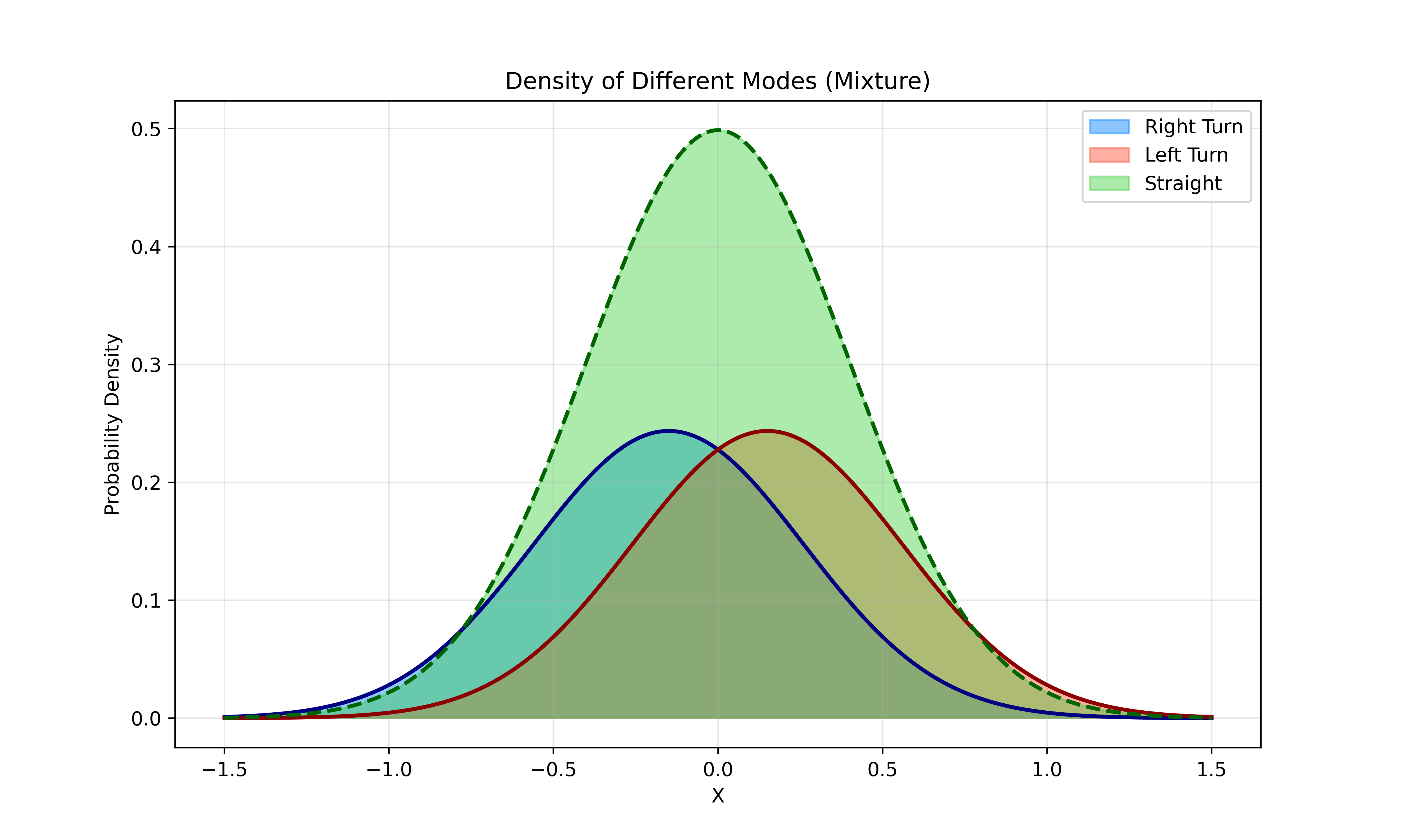
This figure shows that under a specific position, there are three different modes: straight, right turn, and left turn. This makes it hard for the model to learn the correct modes: when positioned to the left, it learns to turn right, and when to the right, it learns to turn left.

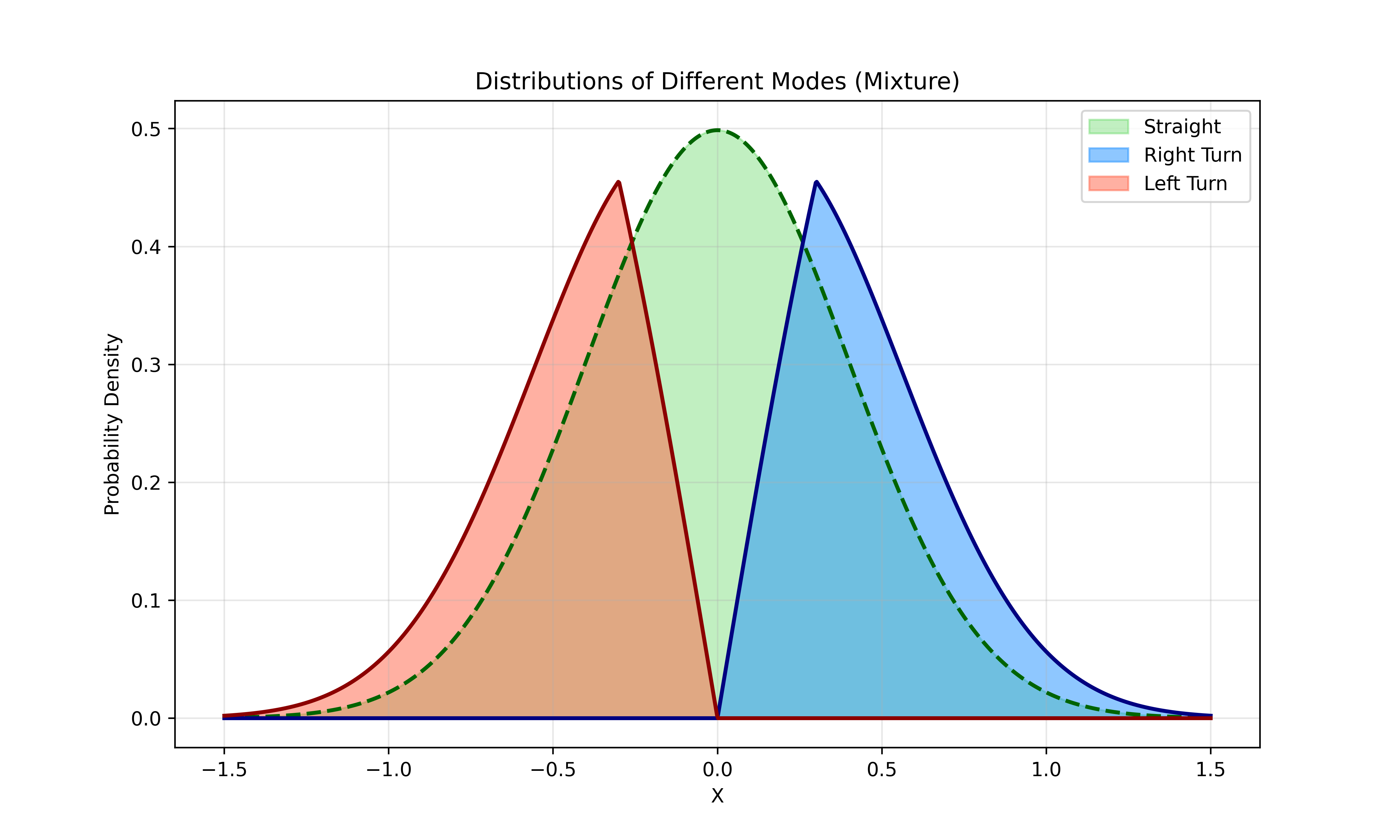
What is worse, there are some undesired modes, e.g., when to the left of the centerline, there are left turn modes. To remove the undesired modes, we can simply add an augmentation rule that when the original position is to the left of the centerline, we only do left shift augmentation, and when the original position is to the right of the centerline, we only do right shift augmentation. Thus, we can compute the distribution of the right turn as below:

$$ \begin{aligned} F_Y(y|\text{right turn}) &= P(Y\le y | X\le 0, \text{Aug}, Z\le 0)P(\text{Aug})\\ &= P(\text{Aug}) * P(X+Z \le y | X\le 0, Z\le 0) \\ &= P(\text{Aug})*\int_{x+z\le y, x \le 0, z\le 0} f_{XZ}(x,z)\mathrm{d}x\mathrm{d}z \\ &= p * \int_{x+z\le y, x \le 0, z\le 0}f_X(x)f_Z(z)\mathrm{d}x\mathrm{d}z \\ &= p * \int_{-\infty}^{0}\int_{-\infty}^{y-z}f_X^{-}(x)f_Z(z)\mathrm{d}x\mathrm{d}z \end{aligned} $$

where

$$ f_X^{-}(x) = \begin{cases} f_X(x), & x \le 0 \\ 0, & x > 0 \end{cases} $$

Thus, the probability density function, $f_Y(y|\text{Right Turn})$, is computed as below:

$$ f_Y(y|\text{Right Turn}) = p * \int_{-\infty}^{0}f_X^{-}(y-z)f_Z(z)\mathrm{d}z $$

Similarly, we have

$$ f_Y(y|\text{Left Turn}) = p * \int_{0}^{\infty}f_X^{+}(y-z)f_Z(z)\mathrm{d}z $$

where

$$ f_X^{+}(x) = \begin{cases} f_X(x), & x \ge 0 \\ 0, & x < 0 \end{cases} $$

and

$$ f_Y(y|\text{Straight}) = f_X(y). $$

If again, $Z\sim \mathcal{U}(-z_0, z_0)$, where $z_0>0$, the probability density function, $f_Y(y|\text{Right Turn})$, is computed as below:

$$ \begin{aligned} f_Y(y|\text{Right Turn}) &= p * \int_{-z_0}^{0}f_X^{-}(y-z)f_Z(z)\mathrm{d}z\\ &=p*\left( -\int_{y+z_0}^{y} f^{-}_X(u)\mathrm{d}u \right)\\ &=p*\left( \int_{y}^{y+z_0}f^{-}_X(u)\mathrm{d}u \right)\\ &=p*\left(\phi^{-}(y+z_0)-\phi^{-}(y)\right) \end{aligned} $$

where

$$ \phi^{-}(x)= \begin{cases} \phi(x) \text{ if } x\le 0 \\ \frac{1}{2} \text{ else} \end{cases} $$

and $\phi(x)$ is the cumulative distribution function of $X$. So, we have the density function conditioned on turning right:

$$ f_Y(y|\text{Right Turn}) = p * \left(\phi^{-}(y+z_0)-\phi^{-}(y)\right)\\ =\begin{cases} \phi(y+z_0) - \phi(y) \text{, } y\le -z_0 \\ \frac{1}{2} - \phi(y) \text{, } -z_0 < y \le 0\\ 0 \text{, else.} \end{cases} $$

Similarly, we can get the density function conditioned on left turn.

In the figure below, we set $X\sim \mathcal{N}(0, 0.4^2)$ and $z_0=0.3$ and plot the three conditional density functions.

That looks better now. Under this augmentation, we do not have confusing modes anymore. But for a regression model, it is not enough. Since regression models tend to learn the mean of the modes. A diffusion model may help here.

Why do people take random uniform augmentation for granted? I think they may think all the trajectories are almost on the centerline. To clarify this point, we set $X\sim\mathcal{N}(0, 0.05)$, $Z\sim\mathcal{U}(-0.3, 0.3)$, and $p=0.5$. We repeat the above two experiments and get the two figures as below

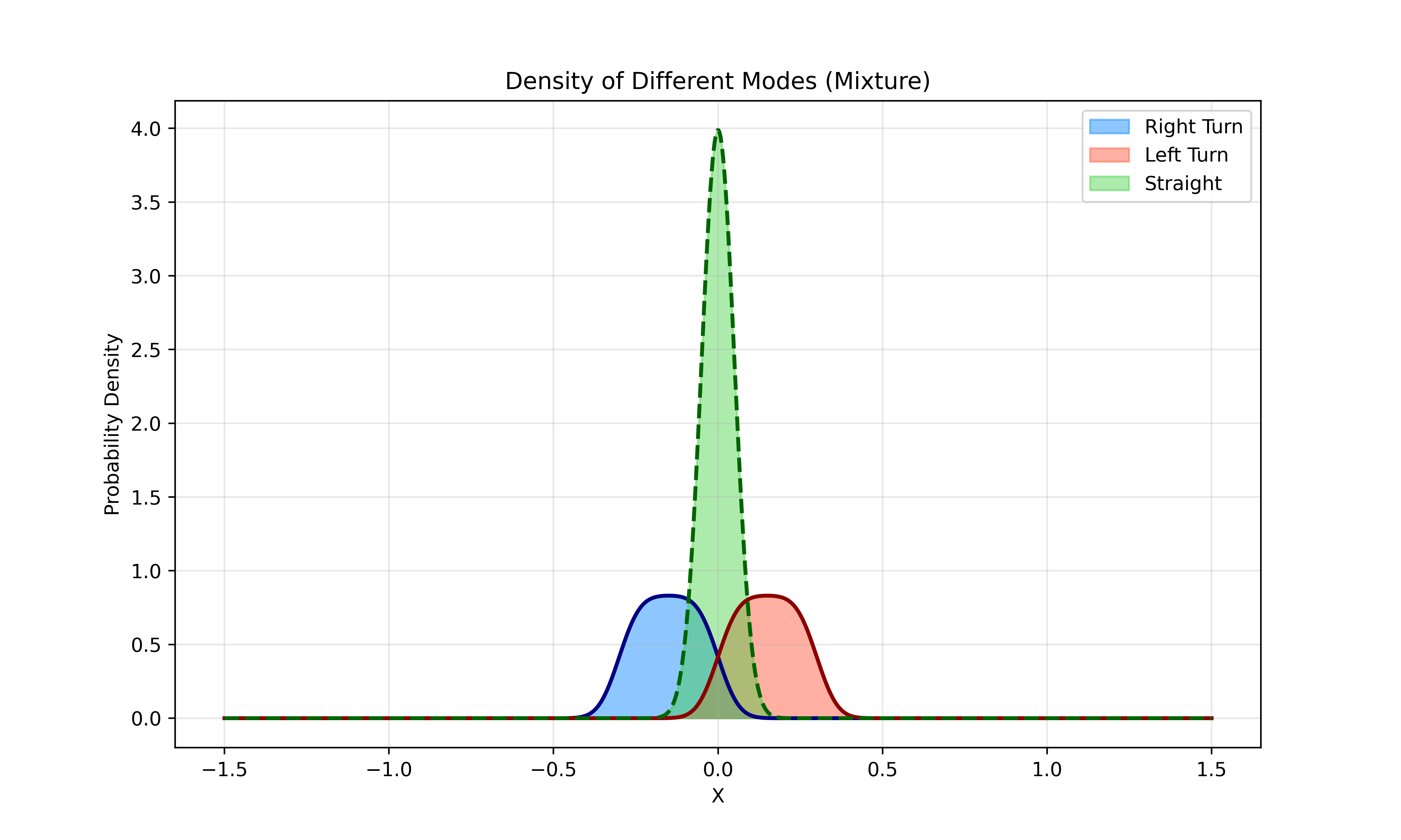
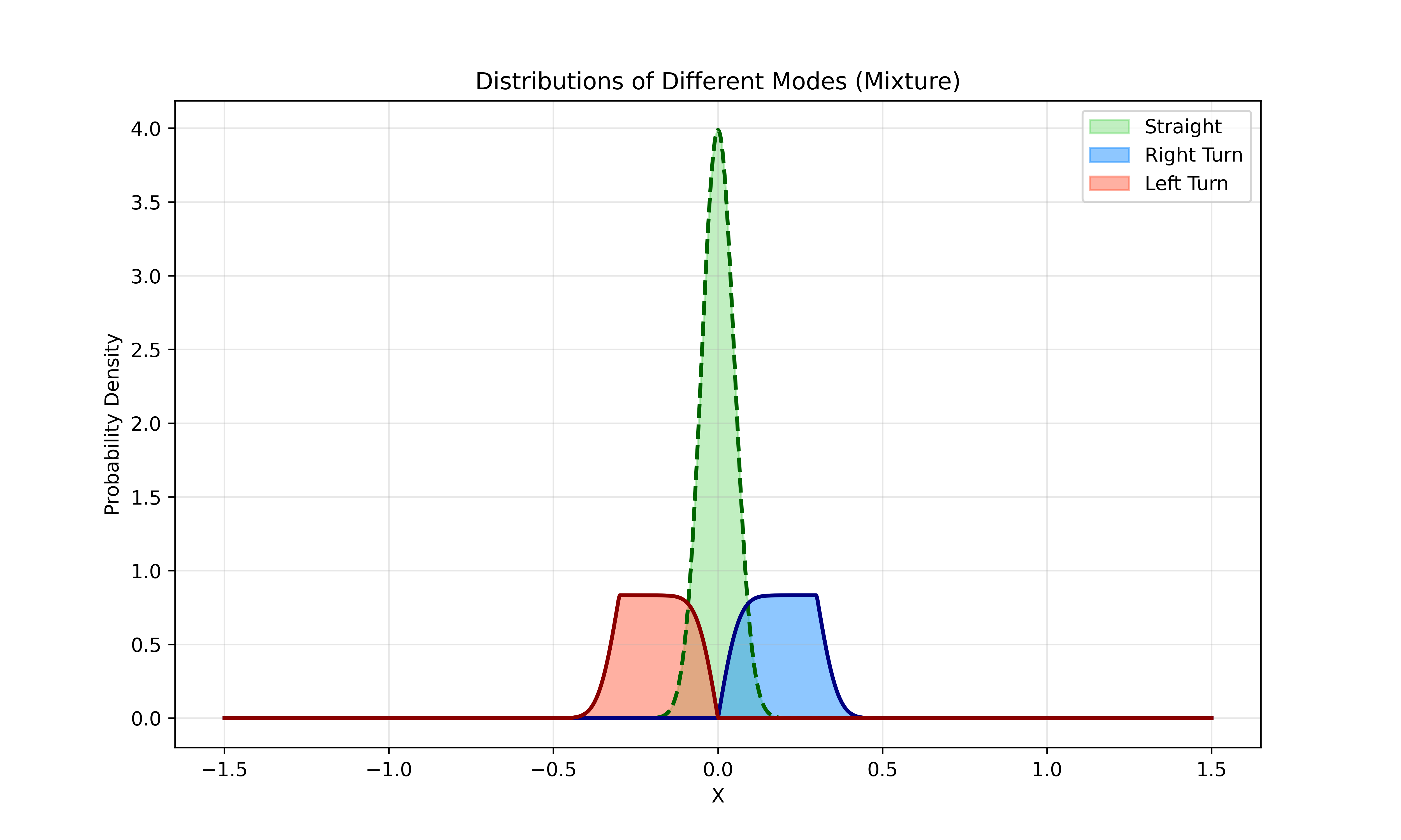
From the above two figures we can see, when the original distribution is near Dirac delta distribution, even simple uniform augmentation works.

The Curvature v.s. Speed

The curvature and speed in the dataset are highly correlated.

Firstly, we will compute the current curvature given the speed and acceleration by

$$ \kappa(t)=\frac{x^\prime(t)y^{\prime\prime}(t)-x^{\prime\prime}(t)y^\prime(t)}{\left(x^\prime(t)^2+y^\prime(t)^2\right)^{3/2}}. $$

Here we keep the sign of the curvature to inform the direction of the turn. Then, we plot the curvature speed of the data samples in the following figure.

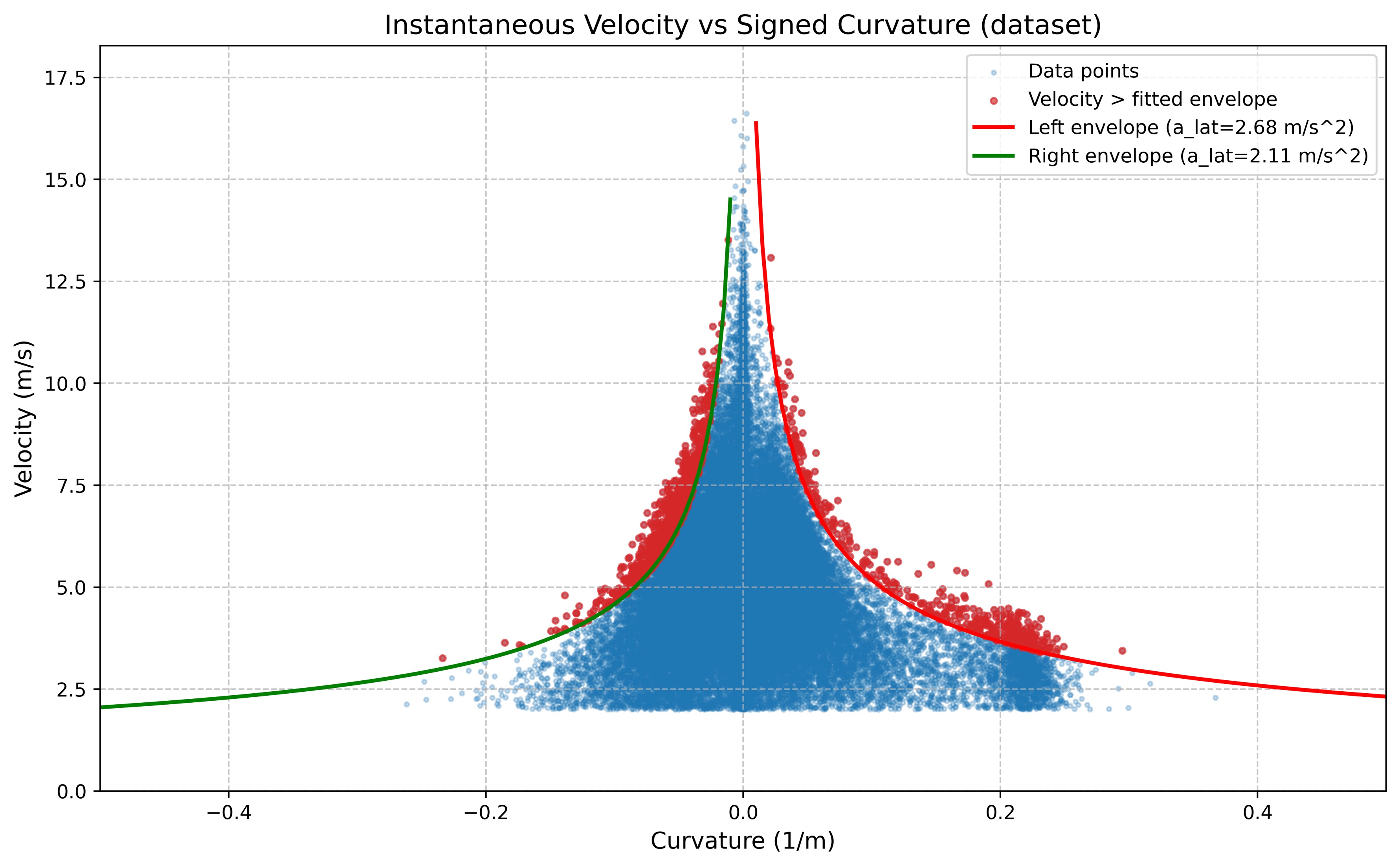
It is clear that the curvature and speed are bounded by a function. In order to compute the upper bound function, we will follow these steps in below.

Firstly, we split the data into two groups based on the sign of the curvatures: Left turn, $\kappa >0$ and right turn, $\kappa \le 0$. Each side is treated as an independent fitting problem to account for potential asymmetries in vehicle performance or scenario distribution.

Secondly, we perform envelope detection. Instead of fitting every raw point, we need to find the maximum speed for each curvature. The curvature range (from 0.01 to 0.5) is divided into 20 bins. In each bin, we calculate the 95th percentile of the velocities. Using the absolute maximum is often too sensitive to noise or outliers. The 95th percentile captures the “reliable” operational boundary of the data.

Thirdly, we need to choose a candidate parameterized function for the boundary function. Here we resort to the vehicle dynamics. The achievable lateral acceleration is bounded by tire-road friction and/or comfort

$$ a_{lat} \le \mu g. $$

We assume a constant maximum lateral acceleration boundary $a_{lat}$, governed by

$$ a_{lat}=v^2\cdot |\kappa|. $$

Instead of complex non-linear optimization, we treat this as a direct calculation. For every envelope point $(v_i, \kappa_i)$ found in the above step, we compute its corresponding lateral acceleration, $a_i=v_i^2\cdot\kappa_i$.

Finally, we need to estimate the parameter $a_{lat}$. If we use the mean, we end up with

$$ \hat{a}_{lat} = \text{mean}(\{a_i\}). $$

In the curvature v.s. speed figure, the red line is the fitted upper bound function. Given a curvature, any speed lower than the upper bound is a plausible speed.