Diffusion models have emerged as a powerful and flexible class of generative models, underpinning recent breakthroughs in image, audio, and scientific data generation. This article offers a gentle, beginner-friendly overview of diffusion models and the related flow matching framework, demystifying their mathematical foundations and practical training procedures. We will delve into the core concepts, guiding equations, and step-by-step training algorithms, aiming to provide readers with both an intuition for how these models work and a roadmap for implementing them in practice. This article serves as notes on papers [1] and [2].
Generative Models
The original motivation behind diffusion models is to generate high-quality, diverse data. To achieve this, we map the observed data distribution to a simple base distribution, sample from the base, and map the samples back to data space. Thus, the goal of a generative model is to learn a mapping between the data and base distributions (in either direction).
Diffusion Models
Flow Matching
We mainly follow tutorial [1] to introduce flow matching and diffusion models.
Flow is a solution to the ODE
$$ \psi : \mathbb{R}^d \times [0,1] \to \mathbb{R}^d, \quad (x_0, t) \mapsto \psi_t(x_0) \tag{2a} $$$$ \frac{d}{dt} \psi_t(x_0) = u_t\bigl(\psi_t(x_0)\bigr) \tag{2b} $$$$ \psi_0(x_0) = x_0 \tag{2c} $$For a given initial condition $X_0 = x_0$, a trajectory of the ODE is recovered via $X_t = \psi_t(X_0)$. Therefore, vector fields, ODEs, and flows are, intuitively, three descriptions of the same object: vector fields define ODEs whose solutions are flows.
Solutions are flows. As with every equation, we should ask: does a solution exist, and if so, is it unique? Under mild assumptions on $u_t$, the answer is “yes” to both:
Theorem 3 (Flow existence and uniqueness)
If $u : \mathbb{R}^d \times [0,1] \to \mathbb{R}^d$ is continuously differentiable with a bounded derivative, then the ODE in (2) has a unique solution given by a flow $\psi_t$. In this case, $\psi_t$ is a diffeomorphism for all $t$, i.e. $\psi_t$ is continuously differentiable with a continuously differentiable inverse $\psi_t^{-1}$.
Simulating an ODE. In general, it is not possible to compute the flow $\psi_t$ explicitly if $u_t$ is not as simple as a linear function. In these cases, one uses numerical methods to simulate ODEs. Fortunately, this is a classical and well researched topic in numerical analysis, and a myriad of powerful methods exist [11]. One of the simplest and most intuitive methods is the Euler method. In the Euler method, we initialize with $X_0 = x_0$ and update via
$$ X_{t+h} = X_t + h\,u_t(X_t) \qquad (t = 0, h, 2h, 3h, \ldots, 1 - h) \tag{4} $$where $h = n^{-1} > 0$ is a step size hyperparameter with $n \in \mathbb{N}$. For this class, the Euler method will be good enough. To give you a taste of a more complex method, let us consider Heun’s method defined via the update rule
$$ X'_{t+h} = X_t + h\,u_t(X_t) \quad\text{(initial guess of new state)} $$$$ X_{t+h} = X_t + \frac{h}{2}\bigl(u_t(X_t) + u_{t+h}(X'_{t+h})\bigr) \quad\text{(update with average u at current and guessed state)} $$Intuitively, Heun’s method is as follows: it takes a first guess $X'_{t+h}$ of what the next step could be but corrects the direction initially taken via an updated guess.
Flow models. We can now construct a generative model via an ODE. Remember that our goal was to convert a simple distribution $p_{\text{init}}$ into a complex distribution $p_{\text{data}}$. The simulation of an ODE is thus a natural choice for this transformation. A flow model is described by the ODE
$$ X_0 \sim p_{\text{init}} \qquad \triangleright\ \text{random initialization} $$$$ \frac{d}{dt} X_t = u_t^\theta(X_t) \qquad \triangleright\ \text{ODE} $$where the vector field $u_t^\theta$ is a neural network $u_t^\theta$ with parameters $\theta$. For now, we will speak of $u_t^\theta$ as being a generic neural network; i.e. a continuous function $u_t^\theta : \mathbb{R}^d \times [0,1] \to \mathbb{R}^d$ with parameters $\theta$. Later, we will discuss particular choices of neural network architectures. Our goal is to make the endpoint $X_1$ of the trajectory have distribution $p_{\text{data}}$, i.e.
$$ X_1 \sim p_{\text{data}} \quad \Leftrightarrow \quad \psi_1^\theta(X_0) \sim p_{\text{data}} $$where $\psi_t^\theta$ describes the flow induced by $u_t^\theta$. Note however: although it is called flow model, the neural network parameterizes the vector field, not the flow. In order to compute the flow, we need to simulate the ODE. In algorithm 1, we summarize the procedure how to sample from a flow model.
Diffusion Models
In eq. (1a). Hence, we need to find an equivalent formulation of ODEs that does not use derivatives. where $R_t(h)$ describes a negligible function for small $h$, i.e. such that $\lim_{h \to 0} R_t(h) = 0$, and in (i) we simply use the definition of derivatives. The derivation above simply restates what we already know: A trajectory $(X_t)_{0 \le t \le 1}$ of an ODE takes, at every timestep, a small step in the direction $u_t(X_t)$. We may now amend the last equation to make it stochastic: A trajectory $(X_t)_{0 \le t \le 1}$ of an SDE takes, at every timestep, a small step in the direction $u_t(X_t)$ plus some contribution from a Brownian motion:
$$ X_{t+h}= X_t + \underbrace{h\,u_t(X_t)}_{\text{deterministic}} + \underbrace{\sigma_t\bigl(W_{t+h} - W_t\bigr)}_{\text{stochastic}}+ \underbrace{h\,R_t(h)}_{\text{error term}}\tag{6} $$where $\sigma_t \ge 0$ describes the diffusion coefficient and $R_t(h)$ describes a stochastic error term such that the standard deviation $\mathbb{E}\bigl[\lVert R_t(h)\rVert^2\bigr]^{1/2} \to 0$ goes to zero for $h \to 0$. The above describes a stochastic differential equation (SDE).
It is common to denote a stochastic differential equation (SDE) in the following symbolic notation:
$$ \mathrm{d}X_t = u_t(X_t)\,\mathrm{d}t + \sigma_t\,\mathrm{d}W_t \tag{7a} $$$$ X_0 = x_0 \tag{7b} $$Theorem 5 (SDE Solution Existence and Uniqueness)
If $u : \mathbb{R}^d \times [0,1] \to \mathbb{R}^d$ is continuously differentiable with a bounded derivative and $\sigma_t$ is continuous, then the SDE in (7) has a solution given by the unique stochastic process $(X_t)_{0 \le t \le 1}$.
Simulating an SDE. If you struggle with the abstract definition of an SDE so far, then don’t worry about it. A more intuitive way of thinking about SDEs is given by answering the question: How might we simulate an SDE? The simplest such scheme is known as the Euler–Maruyama method, and is essentially to SDEs what the Euler method is to ODEs. Using the Euler–Maruyama method, we initialize $X_0 = x_0$ and update iteratively via
$$ X_{t+h} = X_t + h u_t(X_t) + \sqrt{h}\,\sigma_t \epsilon_t, \qquad \epsilon_t \sim \mathcal{N}(0, I_d) \tag{9} $$where $h = n^{-1} > 0$ is a step size hyperparameter for $n \in \mathbb{N}$. In other words, to simulate using the Euler–Maruyama method, we take a small step in the direction of $u_t(X_t)$ as well as add a little bit of Gaussian noise scaled by $\sqrt{h}\,\sigma_t$. When simulating SDEs in this class (such as in the accompanying labs), we will usually stick to the Euler–Maruyama method.
Summary 7 (SDE generative model)
Throughout this document, a diffusion model consists of a neural network $u_t^\theta$ with parameters $\theta$ that parameterize a vector field and a fixed diffusion coefficient $\sigma_t$:
- Neural network: $u^\theta : \mathbb{R}^d \times [0,1] \to \mathbb{R}^d,\ (x,t) \mapsto u_t^\theta(x)$ with parameters $\theta$
- Fixed: $\sigma_t : [0,1] \to [0,\infty),\ t \mapsto \sigma_t$
To obtain samples from our SDE model (i.e. generate objects), the procedure is as follows:
- Initialization: $X_0 \sim p_{\text{init}}$ ▸ Initialize with simple distribution, e.g. a Gaussian
- Simulation: $\mathrm{d}X_t = u_t^\theta(X_t)\,\mathrm{d}t + \sigma_t\,\mathrm{d}W_t$ ▸ Simulate SDE from $0$ to $1$
- Goal: $X_1 \sim p_{\text{data}}$ ▸ Goal is to make $X_1$ have distribution $p_{\text{data}}$
A diffusion model with $\sigma_t = 0$ is a flow model.
$$p_t(x,z) = p_t(x|z)p_{data}(z)$$
as beblow
- sample $z\sim p_{data}(z)$,
- sample $x\sim p_t(x|z)$
Then, we descard $z$. The resulting $x$ is distributed as the marginal $p_t(x)$.
Idealy, we would like to learn a marginal vector field $u_t$ that maps the noise distribution $p_{\text{init}}$ to the data distribution $p_{\text{data}}$. However, it involves learning the marginal distribution $p_t$, which is intractable. Therefore, we need to use the marginalization trick. For marginal vector field, it does not depend on the distribution of the whole data. So, we can construct some conditional vector fields $u_t^{\text{target}}(x \mid z)$ for each data point $z$. By this sepcial construction, we can get closed-form expression of the conditional vector fields. The following theorem shows the relationship between the marginal vector field and the conditional vector field. Indeed we can choose any conditional probability. In practice, we would like to choose the one that is easy to sample and yield trackable targets (vector field).
Theorem 10 (Marginalization trick)
For every data point $z \in \mathbb{R}^d$, let $u_t^{\text{target}}(\cdot \mid z)$ denote a conditional vector field, defined so that the corresponding ODE yields the conditional probability path $p_t(\cdot \mid z)$, viz.,
Then the marginal vector field $u_t^{\text{target}}(x)$, defined by
$$ u_t^{\text{target}}(x) =\int u_t^{\text{target}}(x \mid z) \frac{p_t(x \mid z)\, p_{\text{data}}(z)}{p_t(x)} \, dz, \tag{19} $$follows the marginal probability path, i.e.
$$ X_0 \sim p_{\text{init}}, \qquad \frac{d}{dt} X_t = u_t^{\text{target}}(X_t) \;\;\Rightarrow\;\; X_t \sim p_t \qquad (0 \le t \le 1). \tag{20} $$In particular, $X_1 \sim p_{\text{data}}$ for this ODE, so that we might say “$u_t^{\text{target}}$ converts noise $p_{\text{init}}$ into data $p_{\text{data}}$”.
Why we say $X_1 \sim p_{\text{data}}$? It is due to the fact that we implicitly in the conditional probability states that $p_1(\cdot|z)=\delta_z$ and we have $p_1(x) = \int p_1(x|z)p_{\text{data}}(z)\mathrm{d}z=\int \delta_z\cdot p_{\text{data}}(z)\mathrm{d}z=p_{\text{data}}(z)$.
Here I list some notations for clarification.
| Concept | Notation | Meaning |
|---|---|---|
| Single deterministic solution | $x_t$ | state at time (t) for a fixed $x_0$ |
| Explicit dependence on start | $x(t;x_0)$ | same, but shows dependence on $x_0$ |
| Flow map | $\phi_t(x_0)$ | the function mapping $x_0 \mapsto x_t$ |
| Random state | $X_t$ | $x_t$ when $x_0$ is random |
| Sampling statement | $X_t \sim p_t$ | distribution (law) of $X_t$ is $p_t$ |
A minimal mental model
- Pick initial point $x_0$.
- The ODE defines a path $t\to x_t$. (trajectory)
- Collect all these paths into $x_t=\phi_t(x_0)$. (flow map)
- if $x_0$ is random, call it $X_0$ and the path is $X_t$. (random process)
The following theorem shows the relationship between the vector field and the distribution. It tells that the change of the distribution over time is equal to the probability move according to the vector field.
$$ \partial_t p_t(x) = -\operatorname{div}\big(p_t u_t^{\text{target}}\big)(x) \quad \text{for all } x \in \mathbb{R}^d,\, 0 \le t \le 1, \tag{24} $$
where $\partial_t p_t(x) = \frac{d}{dt} p_t(x)$ denotes the time-derivative of $p_t(x)$ (This is true because we fix $x$ here. It is different from the following Langarangian equation where it focuses on the trajectory $x_t$). Equation 24 is known as the continuity equation. (Note that this is partial differential equation (PDE) instead of ordinary partial equaiton )
where the divergence operator $\operatorname{div}$, is defined as:
$$ \operatorname{div}(v_t)(x) = \sum_{i=1}^d \frac{\partial}{\partial x_i} v_t^{\color{red}{(i)}}(x) \tag{23} $$In the book, [1], there is a typo that they mistakenly omitted the superscript $(i)$ in the divergence operator.
The continuity equation states how the probability distribution changes for fix spatial point using the PDE. We can also evaluate the PDE along the curve, $x=X_t$, to get its Langrangain form.
$$ \begin{aligned} \partial_t p_t(x) &=\sum_i\frac{\partial}{\partial x_i}(p \cdot u_i)\\ &= -\nabla\, p_t(x)^\top u_t(x) - \text{div}\,u_t\cdot p_t(x) \end{aligned} $$$\Rightarrow$
$$ \frac{\partial_t p_t(x)}{p_t(x)} = -\text{div}\,u_t(x) - \frac{\nabla p_t(x)^\top}{p_t(x)}u_t(x) $$$\Rightarrow$
$$ \partial_t \ln p_t(x) = -\text{div}\,u_t(x) - \nabla_{x}\ln p_t(x)^\top u_t(x) $$Further, we have
$$ \begin{aligned} \frac{\mathrm{d}}{\mathrm{d}t}\ln p_t(x) &= \frac{\partial_t p_t(x)}{p_t(x)} + \frac{\partial_x p_t(x)\cdot \partial_t x}{p_t(x)}\\ &=\partial_t \ln p_t(x) + \partial_t x^\top \nabla_x \ln p_t(x)\\ &=-\text{div}\,u(x) \end{aligned} $$In summary, we get another nice continuity equation
$$ \frac{\mathrm{d}}{\mathrm{d}t}\ln p_t(x) =-\text{div}\,u(x) $$Equivalently
$$ \frac{\mathrm{d}}{\mathrm{d}t} p_t(x) =-p_t(x)\text{div}\,u(x) $$We can even compute the probability, $p_t(x)$. By integration both sides of the above equation, we get
$$ \ln p_t(x) - \ln p_0(x)=-\int_0^t \text{div}\,u(x)\,\mathrm{d}t $$Take exponential on both sides we have
$$ p_t(x)=p_0(x_0)\exp\left(-\int_0^t \text{div}\,u_s(x_s)\,\mathrm{d}s\right) $$We can use the continuity equation to derive the relationship between the marginal vector field and the conditional vector field.
We may also see the following form of the theorem
Theorem 13 (SDE extension trick)
Define the conditional and marginal vector fields $u_t^{\text{target}}(x \mid z)$ and $u_t^{\text{target}}(x)$ as before. Then, for diffusion coefficient $\sigma_t \ge 0$, we may construct an SDE which follows the same probability path:
$$ X_0 \sim p_{\text{init}}, \qquad \mathrm{d}X_t =\Big[ u_t^{\text{target}}(X_t) + \frac{\sigma_t^2}{2} \nabla \log p_t(X_t) \Big] \mathrm{d}t + \sigma_t \mathrm{d}W_t \tag{25} $$$$ \Rightarrow\quad X_t \sim p_t \qquad (0 \le t \le 1) \tag{26} $$In particular, $X_1 \sim p_{\text{data}}$ for this SDE. The same identity holds if we replace the marginal probability $p_t(x)$ and vector field $u_t^{\text{target}}(x)$ with the conditional probability path $p_t(x \mid z)$ and vector field $u_t^{\text{target}}(x \mid z)$. Here, we require $\sigma_t \ge 0$. So, we can inject as much as noise but get the same expected distribution.
Theorem 15 (Fokker–Planck Equation)
Let $p_t$ be a probability path and let us consider the SDE
$$ X_0 \sim p_{\text{init}}, \qquad \mathrm{d}X_t = u_t(X_t)\,\mathrm{d}t + \sigma_t\,\mathrm{d}W_t. $$Then $X_t$ has distribution $p_t$ for all $0 \le t \le 1$ if and only if the Fokker–Planck equation holds:
$$ \partial_t p_t(x) = -\operatorname{div}\big(p_t u_t\big)(x) + \frac{\sigma_t^2}{2}\,\Delta p_t(x) \quad \text{for all } x \in \mathbb{R}^d,\; 0 \le t \le 1. \tag{30} $$Summary 17 (Derivation of the Training Target)
The flow training target is the marginal vector field $u_t^{\text{target}}$. To construct it, we choose a conditional probability path $p_t(x\mid z)$ that fulfils $p_0(\cdot \mid z) = p_{\text{init}},\ p_1(\cdot \mid z) = \delta_z$. Next, we find a conditional vector field $u_t^{\text{flow}}(x\mid z)$ such that its corresponding flow $\psi_t^{\text{target}}(x\mid z)$ fulfills
$$ X_0 \sim p_{\text{init}} \;\Rightarrow\; X_t = \psi_t^{\text{target}}(X_0\mid z) \sim p_t(\cdot \mid z), $$or, equivalently, that $u_t^{\text{target}}$ satisfies the continuity equation. Then the marginal vector field defined by
$$ u_t^{\text{target}}(x) =\int u_t^{\text{target}}(x\mid z) \frac{p_t(x\mid z)p_{\text{data}}(z)}{p_t(x)}\,\mathrm{d}z, \tag{32} $$follows the marginal probability path, i.e.,
$$ X_0 \sim p_{\text{init}}, \quad \mathrm{d}X_t = u_t^{\text{target}}(X_t)\,\mathrm{d}t \;\Rightarrow\; X_t \sim p_t \quad (0 \le t \le 1). \tag{33} $$In particular, $X_1 \sim p_{\text{data}}$ for this ODE, so that $u_t^{\text{target}}$ “converts noise into data”, as desired.
Extending to SDEs. For a time-dependent diffusion coefficient $\sigma_t \ge 0$, we can extend the above ODE to an SDE with the same marginal probability path:
$$ X_0 \sim p_{\text{init}}, \quad \mathrm{d}X_t = \Big[ u_t^{\text{target}}(X_t) + \frac{\sigma_t^2}{2}\nabla \log p_t(X_t) \Big] \mathrm{d}t + \sigma_t \mathrm{d}W_t \tag{34} $$$$ \Rightarrow\; X_t \sim p_t \quad (0 \le t \le 1), \tag{35} $$where $\nabla \log p_t(x)$ is the marginal score function
$$ \nabla \log p_t(x) =\int \nabla \log p_t(x\mid z) \frac{p_t(x\mid z)p_{\text{data}}(z)}{p_t(x)}\,\mathrm{d}z. \tag{36} $$Conditional and Marginal Score Functions
In particular, for the trajectories $X_t$ of the above SDE, it holds that $X_1 \sim p_{\text{data}}$, so that the SDE “converts noise into data”, as desired. An important example is the Gaussian probability path, yielding the formulae:
$$ p_t(x\mid z) =\mathcal{N}(x; \alpha_t z, \beta_t^2 I_d) \tag{37} $$$$ u_t^{\text{flow}}(x\mid z) =\left(\dot{\alpha}_t- \frac{\dot{\beta}_t}{\beta_t}\alpha_t \right) z + \frac{\dot{\beta}_t}{\beta_t} x \tag{38} $$$$ \nabla \log p_t(x\mid z) =- \frac{x - \alpha_t z}{\beta_t^2}, \tag{39} $$for noise schedulers $\alpha_t, \beta_t \in \mathbb{R}$: continuously differentiable, monotonic functions such that $\alpha_0 = \beta_1 = 0$, $\alpha_1 = \beta_0 = 1$.
In general, If you define a conditional flow map (or know the sampling method) as $x=\phi_t(z, \epsilon)$. Let us define the random veriable
$$ X_t := \phi_t(z, \epsilon) $$Then we can get $u_t(x|z)$ by taking partial derivative of $X_t$
$$ u_t(x|z) = \partial_t X_t = \partial_t \phi_t(z, \varepsilon) $$$u_t$ is function of $x$. So, we need represent $\varepsilon$ as function of $x$. Thus we get $\varepsilon = \phi_t^{-1}(x, z)$. So, we get the conditional velocity field
$$ u_t(x|z) = \partial_t\left(x, \phi_t^{-1}(x, z)\right) $$Training the Generative Model
We are trying to learn the marginal vector field $u_t^{\text{target}}(x)$. So, our objective is to parameter a neuron network, $v^{\theta}_t(x)$ to approximate $u_t^{\text{target}}(x)$ at every $t$ and $x$. Thus, our cost function is
$$ \mathcal{L}(\theta) = \mathbb{E}_{t, x} \left[ \| v^{\theta}_t(x) - u_t^{\text{target}}(x) \|^2 \right]. $$Here we do not constrain the distribution of $t$. But, a convenient choice is uniform distribution, $t\sim \mathcal{U}(0,1)$. Other choices are possible, e.g., Beta distribution. Since $x = p_t(x) = \int p(x|z)p_{\text{data}}(z)\mathrm{d}z$, we have
$$ L_{\text{FM}}(\theta) = \mathbb{E}_{t\sim \mathcal{U}(0,1), x\sim p_t(x|z), z\sim p_{\text{data}}(z)} \left[ \| v^{\theta}_t(x) - u_t^{\text{target}}(x) \|^2 \right]. $$Theorem 18 The marginal flow matching loss equals the conditional flow matching loss up to a constant. That is
$$ \mathcal{L}_{\text{FM}}(\theta) = \mathcal{L}_{\text{CFM}}(\theta) + C, $$$$ \nabla_\theta \mathcal{L}_{\text{FM}}(\theta) = \nabla_\theta \mathcal{L}_{\text{CFM}}(\theta). $$Hence, minimizing $\mathcal{L}_{\text{CFM}}(\theta)$ with e.g., stochastic gradient descent (SGD) is equivalent to minimizing $\mathcal{L}_{\text{FM}}(\theta)$ in the same fashion. In particular, for the minimizer $\theta^*$ of $\mathcal{L}_{\text{CFM}}(\theta)$, it will hold that $u_t^{\theta^*} = u_t^{\text{target}}$ (assuming an infinitely expressive parameterization).
Algorithm 3 Flow Matching Training Procedure (here for Gaussian CondOT path $p_t(x\mid z) = \mathcal{N}(tz, (1 - t)^2)$)
Require: A dataset of samples $z \sim p_{\text{data}}$, neural network $u_t^\theta$
$$\mathcal{L}(\theta) = \lVert u_t^\theta(x) - (z - \epsilon) \rVert^2$$
(General case: $= \lVert u_t^\theta(x) - u_t^{\text{target}}(x\mid z) \rVert^2$)
7: Update the model parameters $\theta$ via gradient descent on $\mathcal{L}(\theta)$.
8: end for
Algorithm 4 Score Matching Training Procedure for Gaussian probability path
Require: A dataset of samples $z \sim p_{\text{data}}$, score network $s_t^\theta$ or noise predictor $\epsilon_t^\theta$
1: for each mini-batch of data do
2: Sample a data example $z$ from the dataset.
3: Sample a random time $t \sim \text{Unif}_{[0,1]}$.
4: Sample noise $\epsilon \sim \mathcal{N}(0, I_d)$ (General case: $x_t \sim p_t(\cdot \mid z)$)
5: Set $x_t = \alpha_t z + \beta_t \epsilon$
6: Compute loss
Alternatively:
$$ \mathcal{L}(\theta) = \lVert \epsilon_t^\theta(x_t) - \epsilon \rVert^2 $$7: Update the model parameters $\theta$ via gradient descent on $\mathcal{L}(\theta)$.
8: end for
Building an Image Generator
The objective of our network is to learn an mixture of the guided and unguided vector fields.
$$ \tilde{u}_t(x|y) = u_t^{\text{target}}(x) + w b_t \nabla \log p_t(y|x) \\ = u_t^{\text{target}}(x) + w b_t (\nabla \log p_t(x|y) - \nabla \log p_t(x)) \\ = u_t^{\text{target}}(x) - (w a_t x + w b_t \nabla \log p_t(x)) + (w a_t x + w b_t \nabla \log p_t(x|y)) \\ = (1 - w) u_t^{\text{target}}(x) + w u_t^{\text{target}}(x|y) $$Summary 27 (Classifier-Free Guidance for Flow Models)
$$ \tilde{u}_t(x|y) = (1-w)u_t^{\text{target}}(x|\varnothing) + w u_t^{\text{target}}(x|y). \tag{70} $$$$ \mathcal{L}^{\text{CFG}}_{\text{CFM}}(\theta) = \mathbb{E}_{\square}\big\lVert u_t^{\theta}(x|y) - u_t^{\text{target}}(x|z) \big\rVert^2 \tag{71} $$$$ \square = (z,y) \sim p_{\text{data}}(z,y),\quad t \sim \text{Unif}[0,1],\quad x \sim p_t(\cdot|z),\ \text{replace } y = \varnothing \text{ with prob. } \eta. \tag{72} $$In plain English, $\mathcal{L}^{\text{CFG}}_{\text{CFM}}$ might be approximated by
- $(z,y) \sim p_{\text{data}}(z,y)$ — Sample $(z,y)$ from data distribution.
- $t \sim \text{Unif}[0,1]$ — Sample $t$ uniformly on $[0,1]$.
- $x \sim p_t(x|z)$ — Sample $x$ from the conditional probability path $p_t(x|z)$.
- with prob. $\eta$, $y \leftarrow \varnothing$ — Replace $y$ with $\varnothing$ with probability $\eta$.
At inference time, for a fixed choice of $y$, we may sample via
- Initialization: $X_0 \sim p_{\text{init}}(x)$ — Initialize with simple distribution (such as a Gaussian).
- Simulation: $\mathrm{d}X_t = \tilde{u}_t^{\theta}(X_t|y)\,\mathrm{d}t$ — Simulate ODE from $t=0$ to $t=1$.
- Samples: $X_1$ — Goal is for $X_1$ to adhere to the guiding variable $y$.
Recent Advances in Diffusion Models
Back to Basics: Let Denoising Generative Models Denoise
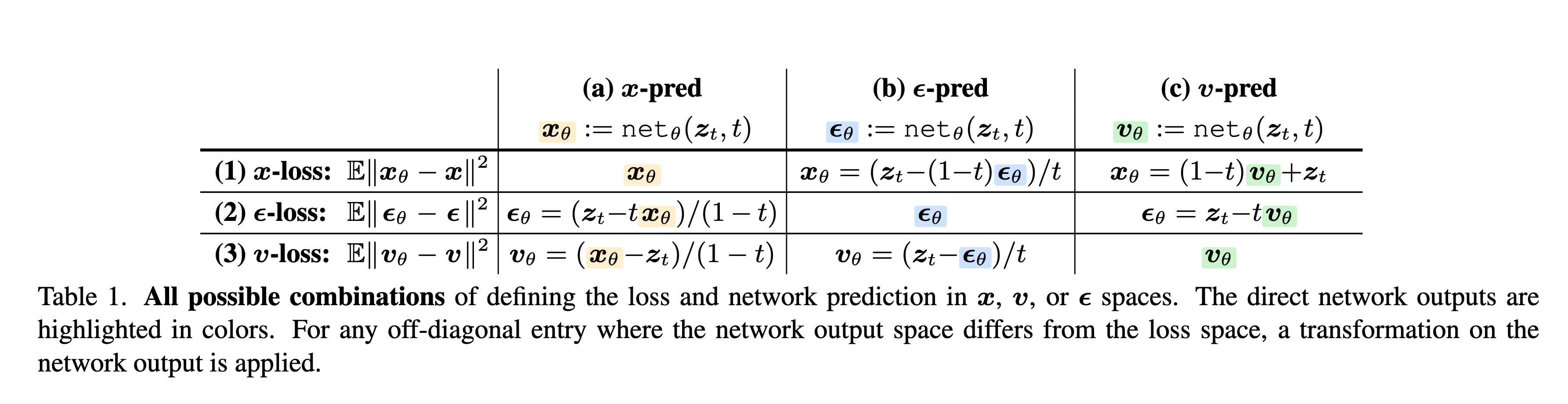
This paper [2] is simple yet inspiring. The toy example in Fig. 2 clearly shows why it is preferable to predict the original data rather than the noise. Table 1 also summarizes how different objectives are related.
Theory
By writing the data distribution as discrete distribution
$$ p(y) = \frac{1}{n} \sum_{i=1}^n \delta_{y^i} $$where $\delta_{y^i}$ is the Dirac delta distribution. Then, we can derive many interesting closed-form expressions [4, 5].
Firstly, we will compute the marginal distribution $X_t \sim p_t(x)$. Let’s assume the conditional probability path is given by
$$ X_t|z \sim \mathcal{N}(\mu_t(z), \sigma_t^2(z)\mathbf{I}_d) $$Then, the marginal distribution is
$$ \begin{aligned} p_t(x) &= \int_z p(z) p_t(x|z) \mathrm{d}z \\ &=\int_z \frac{1}{n} \sum_{i=1}^n \delta_{y^i} \mathcal{N}(x; \mu_t(z), \sigma_t^2(z)\mathbf{I}_d) \mathrm{d}z \\ &=\frac{1}{n} \sum_{i=1}^n \mathcal{N}(x; \mu_t(y^i), \sigma_t^2(y^i)\mathbf{I}_d) \end{aligned} $$It is just a mixture of Gaussians!
Second, we will compute the marginal vector field, $u_t(x)$. Let us reparamterize the conditional variable $X_t$ as
$$ X_t = \alpha_t(z) + \beta_t(z) \varepsilon $$So, we have $\varepsilon = \frac{X_t - \alpha_t(z)}{\beta_t(z)}$ and
$$ \partial_t X_t = \dot{\alpha}_t(z) + \dot{\beta}_t(z) \varepsilon $$Substitute the expression of $\varepsilon$, we have
$$ u_t(x|z) = \frac{\dot{\beta}_t(x)}{\beta_t(z)}\left(x - \alpha_t(z)\right) + \dot{\alpha}_t(z) $$Then, the marginal vector field is
$$ \begin{aligned} u_t(x) &= \int_z u_t(x|z)p_t(z|x) \mathrm{d}z \\ &= \int_z u_t(x|z) \frac{p_t(x|z)p(z)}{\int_z p_t(x|z)p(z)} \mathrm{d}z \\ &= \frac{1}{n} \sum_{i=1}^n u_t(x|y^i) \frac{\mathcal{N}(x; \alpha_t(y^i), \sigma_t^2(y^i)\mathbf{I}_d)}{\frac{1}{n} \mathcal{N}(x; \alpha_t(y^i), \sigma_t^2(y^i)\mathbf{I}_d)}\\ &=\frac{1}{n} \sum_{i=1}^n u_t(x|y^i)\frac{\mathcal{N}\left((x-\alpha_t(y^i))/\sigma_t(y^i);\mathbf{0}, \mathbf{I}_d\right)}{\frac{1}{n} \sum_i\mathcal{N}\left((x-\alpha_t(y^i))/\sigma_t(y^i); \mathbf{0}, \mathbf{I}_d\right)}\\ &=\frac{1}{n} \sum_{i=1}^n u_t(x|y^i)\frac{\exp\left(-\|x-\alpha_t(y^i)\|^2/(2\sigma_t^2(y^i))\right)}{\frac{1}{n} \sum_i\exp\left(-\|x-\alpha_t(y^i)\|^2)/(2\sigma_t^2(y^i)\right)} \end{aligned} $$This is weighted sum of the conditional vector field, where the weights are defined by the exponential of the negative distance to the data samples. Let us look at the example that $\alpha_t(z)=tz$ and $\beta_t(z)=(1-t)$. So that the conditional vector field is
$$ u_t(x|z) = \frac{z-x}{1-t} $$Substituting in the marginal vector filed equation, we have
$$ u_t(x) = \frac{1}{n}\sum_{i=1}^n\frac{y^i - x}{1-t}\cdot\frac{\exp\left(-\|x-t\cdot y^i)\|^2/(2(1-t)^2))\right)}{\frac{1}{n} \sum_i\exp\left(-\|x-t\cdot y^i\|^2)/(2(1-t)^2)\right)} $$References
[1] P. Holderrieth and E. Erives, “An Introduction to Flow Matching and Diffusion Models,” July 12, 2025, arXiv: arXiv:2506.02070. doi: 10.48550/arXiv.2506.02070.
[2] T. Li and K. He, “Back to Basics: Let Denoising Generative Models Denoise,” Nov. 17, 2025, arXiv:2511.13720. doi: 10.48550/arXiv.2511.13720.
[3] Y. Lipman, R. T. Q. Chen, H. Ben-Hamu, M. Nickel, and M. Le, “Flow Matching for Generative Modeling,” Feb. 08, 2023, arXiv: arXiv:2210.02747. doi: 10.48550/arXiv.2210.02747.
[4] W. Gao and M. Li, “How Do Flow Matching Models Memorize and Generalize in Sample Data Subspaces?,” Oct. 31, 2024, arXiv: arXiv:2410.23594. doi: 10.48550/arXiv.2410.23594.
[5] Q. Bertrand, A. Gagneux, M. Massias, and R. Emonet, “On the Closed-Form of Flow Matching: Generalization Does Not Arise from Target Stochasticity,” Dec. 01, 2025, arXiv:2506.03719. doi: 10.48550/arXiv.2506.03719.
[6] T. Bonnaire, R. Urfin, G. Biroli, and M. Mézard, “Why Diffusion Models Don’t Memorize: The Role of Implicit Dynamical Regularization in Training,” Oct. 28, 2025, arXiv: arXiv:2505.17638. doi: 10.48550/arXiv.2505.17638.