Given a starting point, starting direction, ending point, and ending direction, the goal is to generate a feasible and “natural” path that connects the two points. This path should adhere to vehicle dynamics and avoids obstacles. However, it is hard to define what is “natural”.

Path Planning

In this section, we review some classical path planning methods. We ignore the algorithmic details and focus on the resulting path shapes to provide an overview. The demonstration images are generated using the code repository [1].

Classical Paths

A Star and Bidirectional A Star

Depth First Search, Bezier Path, and Model Predictive Trajectory

Voronoi Road Map and Visibility Road Map

Quartic Bezier Spline

We find that the quartic Bezier spline works well for scenarios involving right turns, U-turns, and lane changes [5].

A quartic Bezier spline is defined by five control points, $\mathbf p_0, \mathbf p_1, \mathbf p_2, \mathbf p_3, \mathbf p_4$, with parameters $t \in [0, 1]$, and is given by

$$B(t) = \sum_{i=0}^{4} \binom{4}{i}\, t^i\,(1 - t)^{4-i} \mathbf{p}_i. $$

When $t = 0$, $B(0) = \mathbf{p}_0$ and $t = 1$, $B(1) = \mathbf{p}_4$. Then, $\mathbf{p}_0$ and $\mathbf{p}_4$ are the start and end points, respectively.

Let us define $B_{i,n}(t)=\binom{n}{i}\, t^i\,(1 - t)^{n-i}$. Then, the quartic Bezier spline can be rewritten as:

$$ B(t) = \sum_{i=0}^4 B_{i,4}(t) \mathbf{p}_i. $$

To compute the derivative of the quartic Bezier spline, let us first compute the derivative of $B_{i,n}(t)$:

$$ \frac{d}{dt}B_{i,n}(t) = n \left(B_{i-1,n-1}(t) - B_{i,n-1}(t)\right). $$

Then the derivative of the quartic Bezier spline is:

$$ \begin{aligned} B^\prime(t) &= 4 \sum_{i=1}^4 B_{i-1, 3}(t)\mathbf{p}_{i} - 4 \sum_{i=0}^3 B_{i, 3}(t)\mathbf{p}_{i} \\ &= 4 \sum_{i=0}^3 B_{i, 3}(t)\left(\mathbf{p}_{i+1} - \mathbf{p}_{i}\right). \end{aligned} $$

Observing that

$$ B^\prime(0) = 4 \sum_{i=0}^3 B_{i, 3}(0)\left(\mathbf{p}_{i+1} - \mathbf{p}_{i}\right) = 4 \left(\mathbf{p}_1 - \mathbf{p}_0\right), $$$$ B^\prime(1) = 4 \sum_{i=0}^3 B_{i, 3}(1)\left(\mathbf{p}_{i+1} - \mathbf{p}_{i}\right) = 4 \left(\mathbf{p}_4 - \mathbf{p}_3\right). $$

Smoothness Constraint

Suppose the start unit direction is $\mathbf{d}_0$ and the end unit direction is $\mathbf{d}_4$. To ensure the path curve is smooth at the start and end points, we constrain the path’s first derivative to match the given directions. So, we have $\mathbf{d}_0 \propto \mathbf{p}_1 - \mathbf{p}_0$ and $\mathbf{d}_4 \propto \mathbf{p}_4 - \mathbf{p}_3$. Then, the control points $\mathbf{p}_1$ and $\mathbf{p}_3$ are along the start and end directions, respectively,

$$\mathbf{p}_1 = \mathbf{p}_0 + \alpha \mathbf{d}_0, \quad \mathbf{p}_3 = \mathbf{p}_4 - \beta \mathbf{d}_4,$$

where $\alpha$ and $\beta$ are positive scalars.

Experiments

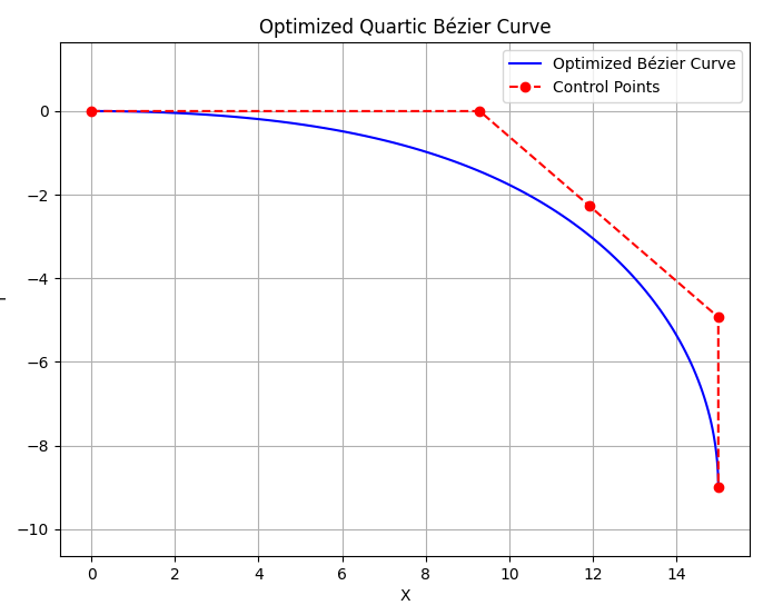
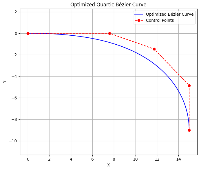
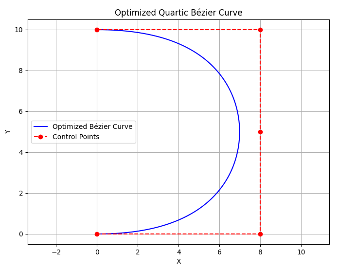
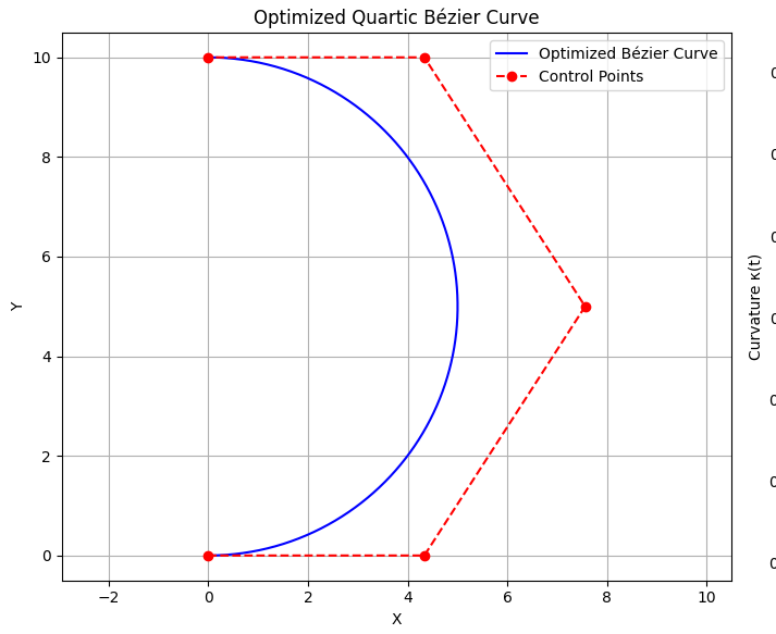
In this experiment, we impose derivative constraints only at the start and end points and explore the resulting path shapes.

We make the starting points at $(0, 0)$ with normalized direction $(1,0)$ We test right turn, U-turn, and lane change, with ending points and directions pairs $[(15, -9), (0, -1)], [(0, 10), (-1, 0)], [(13, 2), (1, 0)]$, respectively.

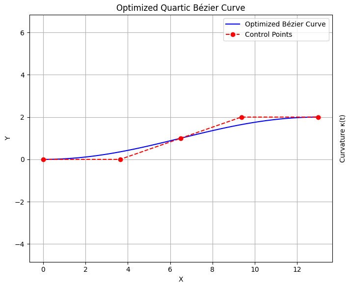
Minimum Variation of Curvature

Defining a “natural” path presents another challenge. The first idea is the model predictive trajectory. However, model predictive trajectory relies on a reference trajectory, which is also difficult to define. After reviewing relevant research, especially regarding model predictive references (e.g., [2,4]), we employ the minimum variation of curvature as our objective to fulfill our requirements. The variation of the curvature is defined as:

$$ V=\int_0^1\left(\frac{d\kappa(t)}{dt}\right)^2\,dt, $$

where $\kappa(t)$ is the curvature of the path at $t$ and can be computed by:

$$ \kappa(t) = \frac{\|B^\prime(t)\times B^{\prime \prime}(t)\|}{\|B^\prime(t)\|^3}, $$

where the second derivative of the quartic Bezier curve is:

$$ B^{\prime \prime}(t) = 12 \sum_{i=0}^{2} B_{i,2}(t)(\mathbf{p}_{i+2} - 2\mathbf{p}_{i+1} + \mathbf{p}_i). $$

Further, we only put maximal curvature constraint as a simplified representation of vehicle dynamic constraints. Meanwhile, we add the distance to obstacles as a hard constraint.

In summary, our optimization problem’s objective is to minimize the variation of the curvature:

$$ \min_{\alpha, \beta, \lambda} \int_0^1\left(\frac{d\kappa(t)}{dt}\right)^2\,dt, $$

with constraints:

1. The curve is smooth at the starting point, meaning the second control point lies along the initial direction:

$$ \mathbf p_1 = \mathbf p_0 + \alpha L \mathbf d_0 $$

the same constraint applies to the end point, leading to the fourth control point,

$$ \mathbf p_3 = \mathbf p_4 - \beta L \mathbf d_4 $$

where $0 < \alpha, \beta < 1$, where $L = \|\mathbf{p}_0 - \mathbf{p}_4 \|$ is the distance between the start and end points.

2. To further simplify the optimization variables, we introduce an optional constraint where the third control point, $\mathbf p_2$, lies on the line segment between $\mathbf p_1$ and $\mathbf p_3$:

$$ \mathbf p_2 = \lambda \mathbf p_1 + (1-\lambda)\mathbf p_3 $$

where $0 \le \lambda \le 1$. Depending on the complexity of the environment, this constraint is optional.

3. Maximal curvature constraint

$$ \kappa(t) \le \kappa_{max} $$

4. Distances to obstacles

$$ d\left(B(t), \mathbf{M}_i\right) \ge r_i, \text{ for all } i = 1, 2, \cdots, M \text{ and } t \in [0, 1] $$

where we model the $i$-th obstacle, $\mathbf{M}_i$, as a circle with radius $r_i$.

Numerical consideration

The variation of curvature constraint is hard to implement directly. We use its numerical approximation:

$$ \frac{d\kappa(t_i)}{dt}\approx \frac{\kappa(t_i) - \kappa(t_{i-1})}{\Delta t} $$

The curvature

$$ \begin{aligned} \kappa(t) &= \frac{\|B^\prime(t)\times B^{\prime \prime}(t)\|}{\|B^\prime(t)\|^3}\\ &= \frac{B_x^\prime(t)B_Y^{\prime \prime} - B_y^\prime(t)B_x^{\prime \prime(t)}}{(B_x^\prime(t)^2 + B_y^\prime(t)^2)^{3/2}} \end{aligned} $$

Algorithm

The algorithm proceeds as follows:

1. Divide parameter, $t$, space, $[0, 1]$, into $N$ equally spaced intervals, with $\{t_i\}_{i=0}^{N}$

2. Compute $\kappa(t_i)$, $\frac{d\kappa(t_i)}{dt}$, and total variation, $V$, numerically

3. Use an optimization algorithm (e.g., Sequential Least-Squares Programming (SLSQP)) to solve the optimization problem.

Experiments

With and Without $\mathbf p_2$ Constraint

Constrained	Unconstrained

Comparison of generated paths. Left column: $\mathbf{p}_2$ constrained. Right column: $\mathbf{p}_2$ unconstrained.

The results indicate that the path generated without the $\mathbf p_2$ constraint appears more natural.

Different Curvature Constraints

Failure Case

Applying non-judiciously chosen initial variables can result in failure.

Specialized $\mathbf{p}_2$ initialization

Summary

To accelerate the optimization, we incrementally add constraints, starting from the simplest, to find a feasible solution.

The optimization variables sets are:

1. $\alpha, \beta, \lambda$
2. $\alpha, \beta, \mathbf{p}_2$

The constraint sets considered are:

1. No direct constraints
2. Maximal curvature
3. Obstacle avoidance

Our workflow is illustrated below: 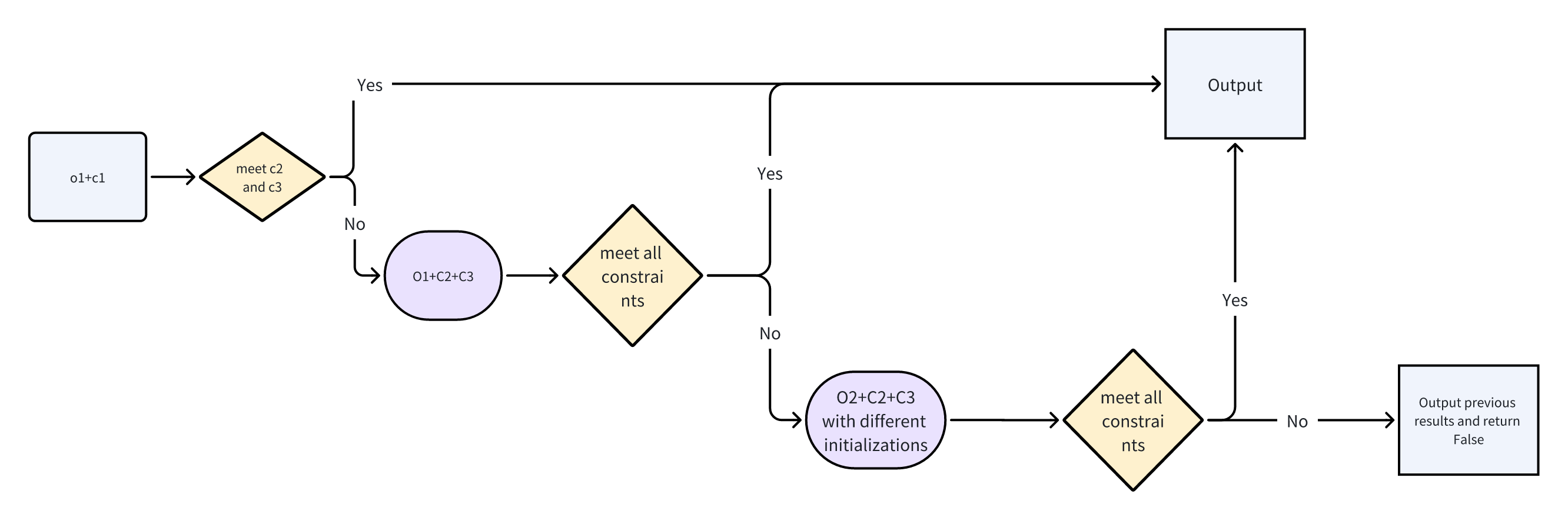where $O_i$ and $C_{j}$, denote the $(i)$th and $(j)$th objective and constraint, respectively.

Some examples are shown below:

Appendix

Ego Vehicle Kinematic Model

In this section, we introduce the kinematic bicycle model [6]. In a kinematic model, we use the velocity, $v$, the position, $(x, y)$, the yaw angle, $\psi$, and the yaw rate, $\dot{\psi}$, to describe the vehicle state. In the meantime, we use the steering angle, $\delta$, and the acceleration, $a$, as the control inputs.

The bicycle model assumes that every point on the vehicle shares the same angular velocity and rotation center, and the front wheel is positioned perpendicular to the line connecting the rotation center and the wheel. With this basic assumption, we can derive the vehicle state and dynamics.

Reference on the Wheel Base

Assume the reference point is located on the wheel base, $B$. Then the basic relationship between position and velocity is:

$$ \begin{aligned} \dot{x} &= v \cos(\beta + \psi), \\ \dot{y} &= v \sin(\beta + \psi), \\ \dot{\psi} &= \frac{v}{|OB|}, \end{aligned} $$

and with geometry equation that $\beta = \angle AOB$, $\delta = \angle AOC$. With this geometry indentities, we can derive the relationships between $\phi, \beta, \delta$.

$$ \begin{aligned} \tan(\beta) &= \frac{|OA|}{\ell_r}, \\ \tan(\delta) &= \frac{|OA|}{\ell_r + \ell_f},\\ \sin(\beta) &= \frac{\ell_r}{|OB|}.\\ \end{aligned} $$

We have $\frac{\tan{\beta}}{\tan{\delta}} = \frac{\ell_r}{\ell_r + \ell_f}$ and $|OB| = \ell_r/ \sin(\beta)$. So, we have the kinematic dynamics:

$$ \begin{aligned} \dot{x} &= v \cos(\beta + \psi), \\ \dot{y} &= v \sin(\beta + \psi), \\ \dot{\psi} &= \frac{v}{\ell_f}\sin(\beta), \\ \dot{v} &= a,\\ \beta &= \arctan\left(\frac{\ell_r}{\ell_f+\ell_r}\tan(\delta)\right), \\ \end{aligned} $$

Reference on the Middle of Rear Axle

If the reference is on the middle of rear axle (point A in the above figure), the vehicle dynamic is:

$$ \begin{aligned} \dot{x} &= v \cos(\psi), \\ \dot{y} &= v \sin(\psi), \\ \dot{\psi} &= \frac{v}{|OA|}, \\ \dot{v} &= a, \end{aligned} $$

with geometry constraints: $\tan{\delta} = \frac{L}{|OA|}$ and $L = \ell_r + \ell_f$ is the wheel base. Thus, the full dynmaic of the vehicle is:

$$ \begin{aligned} \dot{x} &= v \cos(\psi), \\ \dot{y} &= v \sin(\psi), \\ \dot{\psi} &= \frac{v}{L}\tan(\delta), \\ \dot{v} &= a. \end{aligned} $$

As we are dealing in discrete time domain, using the forward Euler method, the state update equation becomes:

$$ X_{k+1} = \begin{bmatrix} x_{k+1} \\ y_{k+1} \\ v_{k+1} \\ \theta_{k+1} \end{bmatrix} = f(x_k, u_k). $$

State Cost

End State Cost

We aim for the terminal state to match a desired state,

$$ \mathbf{x}_e = [x_e, y_e, v_e, \theta_e] $$

So, the end state cost is

$$ (\mathbf{x}-\mathbf{x}_e)^\top\Lambda (\mathbf{x}-\mathbf{x}_e) $$$$\Lambda = \text{diag}(\lambda_x^e, \lambda^e_y, 0, \lambda_\theta^e) $$

Intermediate State Cost

• Acceleration

• Yaw rate

• Desired velocity tracking

Constraints

Low and high acceleration bounds

Low and high yaw rate bounds

Obstacle constraints

Obstacles are represented by points in the plane. So, for each obstacle point, $\mathbf{x}^o_i$, we must have

$$d(\mathbf{x}, \mathbf{x}^o_i) > 0 $$

Linear Quadratic Regulator

Problem

$$ \begin{aligned} \underset{x_1, \dots,x_N, u_1,\dots, u_N }{\text{argmin}} &\quad \frac{1}{2} x_N^T Q_N x_N + \frac{1}{2} \sum_{k=1}^{N-1} x_k^T Q_k x_k + u_k^T R_k u_k \\ s.t. &\quad x_{k+1} = A_k x_t + B_k u_k \end{aligned} $$

Here, the objective function is quadratic with respect to states and controls, and the system transition is linear.

Solution

This problem can be solved using dynamic programming. The solution reveals that the state value function is quadratic, and the optimal policy is linear with respect to the state.

Firstly, the state value function $V(\mathbf{x}_N)$ is known as

$$V(\mathbf{x}_N) = \frac{1}{2}\mathbf{x}_N^\top\mathbf{Q}_N\mathbf{x}_N$$

The state value function, $V(\mathbf{x}_{N-1})$, can be computed by

$$ V(\mathbf{x}_{N-1}) = \min_{\mathbf{u}_{N-1}} \frac{1}{2}\mathbf{x}_{N-1}^\top\mathbf{Q}_{N-1}\mathbf{x}_{N-1} + \frac{1}{2}\mathbf{u}_{N-1}\mathbf{R}_{N-1}\mathbf{u}_{N-1} + V(\mathbf{x}_N) $$

Observing that the function is quadratic with respect to $\mathbf{u}_{N-1}$, taking gradient of the state function with respect to $\mathbf{u}_{N-1}$ and set to zero we have

$$ \begin{aligned} u^*_{N-1} &= -\left( R_{N-1} + B_{N-1}^T S_N B_{N-1} \right)^{-1} B_{N-1}^T S_N A_{N-1} x_{N-1} \\ &\equiv K_{N-1} x_{N-1} \end{aligned} $$

where we define $S_N = Q_N$, and the state value function is

$$ \begin{aligned} V_{N-1}(x_{N-1}) &= \frac{1}{2} x_{N-1}^T Q_{N-1} x_{N-1} + \frac{1}{2} x_{N-1}^T K_{N-1}^T R_{N-1} K_{N-1} x_{N-1} \\ &\quad + \frac{1}{2} \left( A_{N-1} x_{N-1} + B_{N-1} K_{N-1} x_{N-1} \right)^T P_N \left( A_{N-1} x_{N-1} + B_{N-1} K_{N-1} x_{N-1} \right) \\ &= \frac{1}{2} x_{N-1}^T \left( Q_{N-1} + K_{N-1}^T R_{N-1} K_{N-1} + \left( A_{N-1} + B_{N-1} K_{N-1} \right)^T S_N \left( A_{N-1} + B_{N-1} K_{N-1} \right) \right) x_{N-1} \\ &\equiv \frac{1}{2} x_{N-1}^T S_N x_{N-1} \end{aligned} $$

Summary

In the LQR, the objective is quadratic with respect to the state and control, and the optimal control is a linear function of the state.

Iterative Linear Quadratic Regulator

Problem

$$ \begin{aligned} \underset{\mathbf{x}_1,\dots,\mathbf{x}_N, \mathbf{u}_1,\dots,\mathbf{u}_N}{\text{argmin}} &\quad \ell({\mathbf{x}_N})+ \sum_{k=1}^{N-1}\ell(\mathbf{x}_k, \mathbf{u}_k)\\ s.t. & \quad \mathbf{x}_{k+1} = f(\mathbf{x}_k, \mathbf{u}_k) \end{aligned} $$

where the objective function is twice differentiable and the system dynamic is differentiable.

We expand the cost function and system dynamic along a nominal trajectory.

Cost Function

Many cost functions used in iLQR are quadratic. If the cost function is not quadratic, a second-order Taylor series expansion approximates it quadratically. Similarly, the dynamics are linearized using a first-order Taylor expansion. Note that constant terms in the cost expansion are dropped as they do not affect the minimization:

$$ \begin{aligned} J(x_0, U) &= \ell_f(x_N) + \sum_{k=1}^{N-1} \ell(x_k, u_k)\\ &\approx \frac{1}{2} x_N^T Q_N x_N + q_N^T x_N\\ &\quad + \sum_{k=1}^{N-1} \big( \frac{1}{2} x_k^T Q_k x_k + \frac{1}{2} u_k^T R_k u_k + \frac{1}{2} x_k^T H_k u_k + \frac{1}{2} u_k^T H_k^T x_k + q_k^T x_k + r_k^T u_k \big) \end{aligned} $$

System Dynamics

The dynamics are typically provided as continuous-time differential equations. To apply iLQR, these dynamics must first be discretized (e.g., using Euler or Runge-Kutta methods). Here we assume general, non-linear, discretized dynamics:

$$x_{k+1} = f(x_k, u_k)$$

which we linearize using a first-order Taylor-series expansion around nominal state and control trajectories:

$$ X = \{x_0, \dots, x_N\}, U = \{u_0, \dots, u_{N-1}\} $$$$ \begin{aligned} x_{k+1} + \delta x_{k+1} &= f(x_k + \delta x_k, u_k + \delta u_k) \\ &\approx f(x_k, u_k) + \frac{\partial f}{\partial x} \bigg|_{x_k, u_k} (x - x_k) + \frac{\partial f}{\partial u} \bigg|_{x_k, u_k} (u - u_k) \end{aligned} $$$$ \delta x_{k+1} = A(x_k, u_k) \delta x_k + B(x_k, u_k) \delta u_k $$

where $A \equiv \frac{\partial f}{\partial x}$ and $B \equiv \frac{\partial f}{\partial u}$.

Solution

We apply Bellman’s optimality condition to define the state value function and Q value function recursively

$$ \begin{aligned} V_N &= \ell_f(x_N)\\ Q_k &= \min_{u_k} \left\{ \ell(x_k, u_k) + V_{k+1}(f(x_k, u_k)) \right\}\\ V_k &= \min_{u_k} Q_k(x_k, u_k) \end{aligned} $$

We approximate the state value function as locally quadratic near the nominal trajectory:

$$ V_k + \delta V_k = V_k(x_k + \delta x_k) \approx V(x_k) + \left. \frac{\partial V}{\partial x} \right|_{x_k} (x - x_k) + \frac{1}{2} (x - x_k)^T \left. \frac{\partial^2 V}{\partial x^2} \right|_{x_k} (x - x_k) $$$$ \delta V_k(x_k) = s_k^T \delta x_k + \frac{1}{2} \delta x_k^T S_k \delta x_k, $$

where we define $s_k \triangleq \left.\frac{\partial V}{\partial x}\right|_{x_k}$ and $S_k \triangleq \left.\frac{\partial^2 V}{\partial x^2}\right|_{x_k}$.

$$ \begin{aligned} Q_k + \delta Q_k &= Q(x_k + \delta x, u_k + \delta u) \\ &\approx Q(x_k, u_k) + \left. \frac{\partial Q}{\partial x} \right|_{x_k, u_k} (x - x_k) + \left. \frac{\partial Q}{\partial u} \right|_{x_k, u_k} (u - u_k)\\ &+ \frac{1}{2} (x - x_k)^T \left. \frac{\partial^2 Q}{\partial x^2} \right|_{x_k, u_k} (x - x_k) + \frac{1}{2} (u - u_k)^T \left. \frac{\partial^2 Q}{\partial u^2} \right|_{x_k, u_k} (u - u_k) \\ &+ \frac{1}{2} (u - u_k)^T \left. \frac{\partial^2 Q}{\partial u \partial x} \right|_{x_k, u_k} (x - x_k) + \frac{1}{2} (x - x_k)^T \left. \frac{\partial^2 Q}{\partial x \partial u} \right|_{x_k, u_k} (u - u_k) \end{aligned} $$$$ \delta Q_k(x_k, u_k) = \frac{1}{2} \begin{bmatrix} \delta x_k \\ \delta u_k \end{bmatrix}^T \begin{bmatrix} Q_{xx} & Q_{xu} \\ Q_{ux} & Q_{uu} \end{bmatrix} \begin{bmatrix} \delta x_k \\ \delta u_k \end{bmatrix} + \begin{bmatrix} Q_x \\ Q_u \end{bmatrix}^T \begin{bmatrix} \delta x_k \\ \delta u_k \end{bmatrix} $$

We define the following variables using matrix calculus:

$$ \begin{aligned} Q_x &= \ell_x + s_{k+1} A_k \\ Q_u &= \ell_u + s_{k+1} B_k \\ Q_{xx} &= \ell_{xx} + A_k^T S_{k+1} A_k\\ Q_{uu} &= \ell_{uu} + B_k^T S_{k+1} B_k\\ Q_{ux} &= \ell_{ux} + B_k^T S_{k+1} A_k \end{aligned} $$

and using the fact the $Q_{ux} = Q_{xu}^T$, which gives us all the values needed to calculate the next step. We can show this by combining Equations 11 and 12:

By following a dynamic-programming approach, we can solve the tail problem for $V_N(x)$ for a problem with $N$ time steps. In order to solve the detail, we define $\delta V$ as the deviation from the optimal value: with $s_N$ and $S_N$ defined as follows, given the cost function in Equation 7:

$$ \begin{aligned} s_N &\equiv \left. \frac{\partial V}{\partial x} \right|_{x_N}\\ &= \left. \frac{\partial}{\partial x} \left( \frac{1}{2} (x - x_f)^T Q_f (x - x_f) \right) \right|_{x_N}\\ &= \left. \frac{\partial}{\partial x} \left( \frac{1}{2} x^T Q_f x - x_f^T Q_f x + \frac{1}{2} x_f^T Q_f x_f \right) \right|_{x_N}\\ &= Q_f x_N - Q_f x_f \\ &= Q_f (x_N - x_f) \end{aligned} $$$$ \begin{aligned} S_N &\equiv \left. \frac{\partial^2 V}{\partial x^2} \right|_{x_N}\\ &= \left. \frac{\partial}{\partial x} \left( Q_f (x - x_f) \right) \right|_{x_N}\\ &= Q_f \end{aligned} (Q_f = Q_f^T) $$

Solving the Dynamic Programming Problem

After solving the tail sub-problem, we can then apply the principle of optimality and define the process for solving for the $k$th time step given the values at the $k+1$th time step.

$$ \begin{aligned} V_k &= \min_{u_k} \{\ell(x_k, u_k) + V_{k+1}(f(x_k, u_k))\}\\ &= \min_{u_k} \{Q_k(x_k, u_k)\}\\ \delta V &= \min_{\delta u} \{\delta Q(x, u)\}\\ &= \min_{\delta u} \{Q_x \delta x + Q_u \delta u + \frac{1}{2} \delta x^T Q_{xx} \delta x + \frac{1}{2} \delta u^T Q_{uu} \delta u + \frac{1}{2} \delta x^T Q_{xu} \delta u + \frac{1}{2} \delta u^T Q_{ux} \delta x\} \end{aligned} $$$$ \frac{\partial \delta Q}{\partial \delta u} = Q_u + \frac{1}{2} Q_{ux} \delta x + \frac{1}{2} Q_{xu}^T \delta x + Q_{uu} \delta u = 0 $$$$ \Rightarrow \delta u^* = -Q_{uu}^{-1} (Q_{ux} \delta x_k + Q_u) = K \delta x + d $$

So,

$$ \begin{aligned} d_k &= -Q_{uu}^{-1} Q_u \\ K_k &= -Q_{uu}^{-1} Q_{ux} \end{aligned}. $$

After calculating the optimal control as a function of the next time step we can plug it back into Equation (1)

$$ \delta Q_k(x_k, u_k) = \frac{1}{2} \begin{bmatrix} \delta x_k \\ K \delta x + d \end{bmatrix}^T \begin{bmatrix} Q_{xx} & Q_{xu} \\ Q_{ux} & Q_{uu} \end{bmatrix} \begin{bmatrix} \delta x_k \\ K \delta x + d \end{bmatrix} \begin{bmatrix} Q_x \\ Q_u \end{bmatrix}^T \begin{bmatrix} \delta x_k \\ K \delta x + d \end{bmatrix} $$

By equating the result with Equation we get

$$\Delta V = \frac{1}{2} d^T Q_{uu} d + d^T Q_u$$$$s = Q_x + K^T Q_{uu} d + K^T Q_u + Q_{xu}^T d$$$$S = Q_{xx} + K^T Q_{uu} K + K^T Q_{ux} + Q_{ux}^T K$$

Forward Pass

Since the dynamics and the cost function are only approximated at each time step, it is necessary to iteratively solve the previous problem to successively get closer to the local minimum. After each backward pass solving for the optimal correction in control values, $\delta u_k^*$, these values are used to calculate a new state trajectory ( $X$) from the nominal trajectories $\bar{X}, \bar{U}$, often referred to as a ‘‘rollout’’. The $\alpha$ term is used for a line search. This is done using the following algorithm:

$$\delta x = x_k - \bar{x}_k$$$$ \begin{aligned} u_k &= \bar{u}_k + \delta u_k^* \\ &= \bar{u}_k + K_k \delta x_k + \alpha d_k \end{aligned} $$$$ x_{k+1} = f(x_k, u_k) $$

where $\alpha$ is the step size, typically used to perform a simple line search.

Summary

The system dynamic is linearized and the objective function is expanded by the second order Taylor series.

Constrained Iterative Linear Quadratic Regulator

Discrete-time Finite-horizon Motion Planning Problem

$$ \begin{aligned} \arg \min_{x, u} &\quad \left\{ \phi(x_N) + \sum_{k=0}^{N-1} L^k(x_k, u_k) \right\} \\ \text{s.t.} & \quad x_{k+1} = f^k(x_k, u_k), \quad k = 0, 1, \dots, N-1 \\ &\quad x_0 = x_{\text{start}} \\ &\quad g^k(x_k, u_k) < 0, \quad k = 0, 1, \dots, N-1 \\ &\quad g^N(x_N) < 0 \end{aligned} $$

Assumption 1: The system dynamic equation constraints are the only constraints in the problem.

Assumption 2: The inequality constraints are separated to different time steps.

Assumption 3: All the functions in the problem have continuous first and second order derivatives.

Handle Constraints

For inequality constraints, we use the barrier function to shape the constraints:

$$b(g(x, u)) = -\frac{1}{t} \log(-g(x, u))$$

Algorithm

References

[1] https://github.com/AtsushiSakai/PythonRobotics

[2] J. Chen, W. Zhan, and M. Tomizuka, “Autonomous driving motion planning with constrained iterative LQR,” IEEE Transactions on Intelligent Vehicles, vol. 4, no. 2, pp. 244–254, Jun. 2019.

[3] https://github.com/pparmesh/Constrained_ILQR/tree/master/scripts

[4] J. Chen, W. Zhan, and M. Tomizuka, “Constrained iterative LQR for on-road autonomous driving motion planning,” in Proc. 2017 IEEE 20th Int. Conf. Intell. Transp. Syst. (ITSC), Yokohama, Japan, Oct. 2017, pp. 2232–2238.

[5] “Bézier curve,” Wikipedia, The Free Encyclopedia, [Online]. Available: https://en.wikipedia.org/wiki/B%C3%A9zier_curve.

[6] J. Kong, M. Pfeiffer, G. Schildbach, and F. Borrelli, “Kinematic and dynamic vehicle models for autonomous driving control design,” in 2015 IEEE Intelligent Vehicles Symposium (IV), Jun. 2015, pp. 1094–1099. doi: 10.1109/IVS.2015.7225830.

[7] B. E. Jackson, “AL-iLQR Tutorial,” 2019. [Online]. Available: https://bjack205.github.io/papers/AL_iLQR_Tutorial.pdf

[8] B. E. Jackson, “iLQR Tutorial,” 2019. [Online]. Available: https://rexlab.ri.cmu.edu/papers/iLQR_Tutorial.pdf