This article develops end-of-line (EOL) camera extrinsic calibration and calibration-board placement for autonomous-vehicle camera rigs, including bird’s-eye-view applications.
There are two linked optimization problems: estimate camera and board poses from measurements, then choose physical board positions and orientations that make the camera estimates more precise. Camera intrinsics are assumed known, and absolute extrinsics require a world-frame anchor.
The presentation follows this order:
- General calibration problem formulation: variables, coordinate conventions, measurements, priors, and identifiability.
- Solver: sparse factor-graph bundle adjustment for the pose estimates.
- Board-position and orientation optimization formulation: camera uncertainty, design variables, constraints, and optimization methods.
- Experiments from simple to complex: one camera and one board, two-camera cases, a multi-camera workspace, and a vehicle rig.
Geometric preprocessing, ray-plane derivations, and optional design formulations are collected in appendices. The detailed ADMM formulation and solver benchmarks remain in the independent comparison.
1. General Calibration Problem Formulation
For multiple boards and cameras, the observation structure should be defined at the marker-point level. Since each camera may see only a subset of the markers on a board, the primitive observation is a camera-point edge:
$$ (c,p)\in\mathcal E \quad\Longleftrightarrow\quad \text{camera }c\text{ observes marker point }p. $$A board-camera graph is only a compressed graph obtained after grouping all observed points on the same board. The general model uses known board-frame marker coordinates, measured world-frame marker coordinates when available, and image observations. Reprojection residuals share the corresponding physical board pose; the primitive measurements remain camera-point observations.
First define the estimation problem independently of its solver or the eventual board-placement design.
1.1 Sets and Observation Graph
Let there be $B$ boards and $C$ cameras.
Boards:
$$ \mathcal B=\{1,\dots,B\}. $$Cameras:
$$ \mathcal C=\{1,\dots,C\}. $$Board $b$ has known marker points:
$$ \mathcal I_b=\{1,\dots,N_b\}. $$Marker $i$ on board $b$ has known board-frame coordinate:
$$ q_{bi}\in\mathbb R^3. $$For a planar checkerboard or marker board, usually
$$ q_{bi}= \begin{bmatrix} x_{bi}\\ y_{bi}\\ 0 \end{bmatrix}. $$Define the global point set:
$$ \mathcal P= \{p=(b,i): b\in\mathcal B,\ i\in\mathcal I_b\}. $$For point $p=(b,i)$, define
$$ \beta(p)=b $$as the board containing point $p$, and define
$$ q_p=q_{bi}. $$The camera-point observation graph is
$$ \boxed{ \mathcal G=(\mathcal C\cup\mathcal P,\mathcal E), } $$where
$$ \boxed{ (c,p)\in\mathcal E \quad\Longleftrightarrow\quad \text{camera }c\text{ observes point }p. } $$For each observation edge $(c,p)$, the measured image point is
$$ u_{cp}\in\mathbb R^2. $$Camera $c$ has known intrinsic matrix
$$ K_c. $$Define the neighborhoods:
$$ \mathcal N(c)=\{p:(c,p)\in\mathcal E\}, $$$$ \mathcal N(p)=\{c:(c,p)\in\mathcal E\}, $$$$ \mathcal P_b=\{p\in\mathcal P:\beta(p)=b\}. $$1.2 Pose Variables and Coordinate Convention
Use a uniform local-to-world pose convention for both boards and cameras. $T^B_b$ denotes the pose of board $b$, and $T^C_c$ denotes the pose of camera $c$.
For board $b$:
$$ \boxed{ T^B_b= \begin{bmatrix} R^B_b & t^B_b\\ 0 & 1 \end{bmatrix} \in SE(3) } $$maps board-local coordinates to world coordinates:
$$ \boxed{ \bar X_p^W= T^B_{\beta(p)}\bar q_p. } $$Here
$$ \bar q_p= \begin{bmatrix} q_p\\ 1 \end{bmatrix}. $$Define the Euclidean extraction matrix
$$ P_3= \begin{bmatrix} I_3 & 0 \end{bmatrix}. $$Equivalently,
$$ \boxed{ X_p^W= P_3\bar X_p^W= R^B_{\beta(p)} q_p+t^B_{\beta(p)}. } $$For camera $c$:
$$ \boxed{ T^C_c = \begin{bmatrix} R^C_c & t^C_c\\ 0 & 1 \end{bmatrix} \in SE(3) } $$maps camera-local coordinates to world coordinates. Therefore, to project a world point into camera $c$, use the inverse camera pose:
$$ \boxed{ \bar X_{cp}^C = (T^C_c)^{-1}\bar X_p^W. } $$where $\bar X_p^W=[(X_p^W)^\top,1]^\top$.
Explicitly,
$$ (T^C_c)^{-1} = \begin{bmatrix} (R^C_c)^{\top} & -(R^C_c)^{\top}t^C_c\\ 0 & 1 \end{bmatrix}, $$and
$$ \boxed{ X_{cp}^C = (R^C_c)^{\top} \left( X_p^W-t^C_c \right). } $$This is consistent with treating both the board and camera variables as local-to-world poses. The usual computer-vision world-to-camera extrinsic still appears, but now it is written explicitly as $(T^C_c)^{-1}$.
1.3 Projection Model
For point $p=(b,i)$, the homogeneous world coordinate is
$$ \boxed{ \bar X_p^W = T^B_{\beta(p)}\bar q_p. } $$The camera-coordinate point is
$$ \boxed{ \bar X_{cp}^C = (T^C_c)^{-1}T^B_{\beta(p)}\bar q_p. } $$and its Euclidean coordinate is
$$ \boxed{ X_{cp}^C = P_3 (T^C_c)^{-1}T^B_{\beta(p)}\bar q_p \in\mathbb R^3. } $$The projected pixel is
$$ \boxed{ \hat u_{cp} = \Pi\left( K_cX_{cp}^C \right). } $$If
$$ X_{cp}^C= \begin{bmatrix} X\\Y\\Z \end{bmatrix}, $$then, for a standard pinhole model,
$$ \boxed{ \hat u_{cp} = \begin{bmatrix} f_{x,c}X/Z+c_{x,c}\\ f_{y,c}Y/Z+c_{y,c} \end{bmatrix}. } $$These pinhole equations assume undistorted image coordinates. For fisheye or strongly distorted automotive cameras, replace $\Pi(K_cX)$ by the calibrated camera projection model.
It is useful to define the shorthand
$$ \pi_c(X^W;T^C_c) = \Pi\left(K_cP_3(T^C_c)^{-1}\bar X^W\right), $$where $\bar X^W=[(X^W)^\top,1]^\top$. The reprojection residual is
$$ \boxed{ r_{cp}(T^C_c,T^B_{\beta(p)}) = \Pi\left( K_c P_3 (T^C_c)^{-1} T^B_{\beta(p)} \bar q_p \right)-u_{cp}. } $$If the image measurement covariance is
$$ \Sigma_{u,cp}\in\mathbb R^{2\times2}, $$the whitened residual is
$$ \boxed{ e_{cp}(T^C_c,T^B_{\beta(p)}) = \Sigma_{u,cp}^{-1/2} \left[ \Pi\left( K_c P_3 (T^C_c)^{-1} T^B_{\beta(p)} \bar q_p \right) - u_{cp} \right]. } $$1.4 Board and World Measurement Priors
In the original EOL setup, some board marker coordinates may be measured in the world frame. Let
$$ z_p\in\mathbb R^3 $$be the measured world coordinate of point $p$. Define the set of points with world measurements as
$$ \mathcal Z\subseteq\mathcal P. $$The board/world residual is
$$ \boxed{ r^z_p(T^B_{\beta(p)}) = R^B_{\beta(p)} q_p+t^B_{\beta(p)}-z_p. } $$With covariance
$$ \Sigma_{z,p}, $$the board prior term is
$$ \boxed{ \phi_b(T^B_b) = \frac12 \sum_{p\in\mathcal P_b\cap\mathcal Z} \left\| R^B_b q_p+t^B_b-z_p \right\|_{\Sigma_{z,p}^{-1}}^2. } $$You may also have camera pose priors, rig priors, or a fixed reference camera. Write those directly on the camera pose. Let $\bar T^C_c$ be the prior or nominal camera pose. The operator
$$ \operatorname{Log}: SE(3)\rightarrow\mathbb R^6 $$is the Lie-group logarithm that converts a relative pose into a 6D tangent-vector error, usually ordered as three translation components and three rotation components. For example:
$$ \boxed{ \psi_c(T^C_c) = \frac12 \left\| \operatorname{Log} \left( (\bar T^C_c)^{-1}T^C_c \right) \right\|_{\Sigma_c^{-1}}^2. } $$1.5 Centralized Calibration Objective
The cleanest problem is:
$$ \boxed{ \begin{aligned} \min_{\{T^B_b\},\{T^C_c\}} &\quad \sum_{(c,p)\in\mathcal E} \frac12 \left\| \Sigma_{u,cp}^{-1/2} \left[ \Pi\left( K_c P_3 (T^C_c)^{-1} T^B_{\beta(p)} \bar q_p \right) - u_{cp} \right] \right\|^2 \\ &\quad+ \sum_{b\in\mathcal B}\phi_b(T^B_b) + \sum_{c\in\mathcal C}\psi_c(T^C_c). \end{aligned} } \tag{P} $$This is the point-level multi-board, multi-camera bundle-adjustment problem.
The graph edge is $(c,p)$, but the residual depends on
$$ T^C_c \quad\text{and}\quad T^B_{\beta(p)}. $$So the raw observation graph is camera-point, while the variable graph is camera-board because each point is rigidly attached to a board.
This shared board-generated point is how multi-camera consistency enters the bundle-adjustment problem. If two cameras $c_1$ and $c_2$ observe the same point $p$, both reprojection residuals use the same world point
$$ X_p^W=R^B_{\beta(p)} q_p+t^B_{\beta(p)}. $$Thus the two camera observations are coupled through the same board pose and the same physical marker point, rather than through two independent 3D point variables or an extra pairwise cross-camera residual.
With the uniform local-to-world convention, the board-to-camera relative transform is
$$ \boxed{ T_{CB}^{(c,b)} = (T^C_c)^{-1}T^B_b. } $$This maps board $b$’s local coordinates into camera $c$’s local coordinates, so the projection can also be written as
$$ \boxed{ \hat u_{cp} = \Pi \left( K_c P_3 T_{CB}^{(c,\beta(p))} \bar q_p \right). } $$1.6 Gauge Freedom and Identifiability
Without an absolute anchor, each connected component has an $SE(3)$ gauge freedom.
For any
$$ H\in SE(3), $$the transformation
$$ \boxed{ (T^B_b)'=HT^B_b, } $$$$ \boxed{ (T^C_c)'=HT^C_c } $$leaves every relative camera-board projection unchanged:
$$ ((T^C_c)')^{-1}(T^B_b)' = (HT^C_c)^{-1}(HT^B_b) = (T^C_c)^{-1}H^{-1}HT^B_b = (T^C_c)^{-1}T^B_b. $$Therefore, every connected component needs at least one of the following:
$$ \text{one fixed board pose,} $$$$ \text{one fixed camera pose,} $$$$ \text{sufficient world-frame board-point measurements,} $$or
$$ \text{sufficient camera/rig priors.} $$Connectivity alone is not enough. The observations must also be geometrically nondegenerate: enough non-collinear board points, reasonable viewing angles, positive depth, and no nearly rank-deficient configurations.
2. Solver: Sparse Factor-Graph Bundle Adjustment
With the measurement model and gauge fixed, the solver estimates the poses for a given set of observations. It does not yet decide where to move the physical boards.
2.1 Solver Choice
Sparse factor-graph bundle adjustment is the recommended solver for this centralized EOL calibration problem. The detailed ADMM derivation, including point-copy and pose-copy consensus variants, has been moved to ADMM vs. Factor-Graph Bundle Adjustment for Multi-Camera Calibration.
2.2 Factor-Graph Structure
The centralized problem is also a factor graph.
Variables:
$$ \{T^B_b\}_{b=1}^B, \qquad \{T^C_c\}_{c=1}^C. $$Factors:
$$ f_{cp}(T^C_c,T^B_{\beta(p)}) $$for every observation edge $(c,p)\in\mathcal E$.
Board priors:
$$ \phi_b(T^B_b). $$Camera priors:
$$ \psi_c(T^C_c). $$GTSAM describes factor graphs as bipartite graphs connecting factors to the variables they depend on, and emphasizes that such sparse structure is exploited by nonlinear optimization methods.
This is arguably the cleanest implementation model: one factor per camera-point observation, with the point’s board membership determining which board pose variable the factor touches.
2.3 Sparse Updates and Schur Elimination
Solve the centralized objective using sparse nonlinear least squares over camera and board pose increments.
The problem is exactly:
$$ \boxed{ \begin{aligned} \min_{\{T^B_b\},\{T^C_c\}} &\quad \sum_{(c,p)\in\mathcal E} \frac12 \left\| \Sigma_{u,cp}^{-1/2} \left[ \Pi\left( K_c P_3 (T^C_c)^{-1} T^B_{\beta(p)} \bar q_p \right) - u_{cp} \right] \right\|^2 \\ &\quad+ \sum_b\phi_b(T^B_b) + \sum_c\psi_c(T^C_c). \end{aligned} } $$Use pose increments:
$$ T^B_b\leftarrow \exp(\delta\xi_b^\wedge)T^B_b, $$$$ T^C_c\leftarrow \exp(\delta\eta_c^\wedge)T^C_c. $$Linearize every residual:
$$ e_{cp} \approx e_{cp}^0 + J_{B,cp}\delta\xi_{\beta(p)} + J_{C,cp}\delta\eta_c. $$Stack all residuals and solve the damped normal equations:
$$ \boxed{ \left(J^\top J+\lambda D\right)\delta = - J^\top r. } $$Each residual touches only one board pose and one camera pose. Therefore the normal matrix has sparse block structure:
$$ \begin{bmatrix} H_{CC} & H_{CB}\\ H_{BC} & H_{BB} \end{bmatrix} \begin{bmatrix} \delta C\\ \delta B \end{bmatrix} = - \begin{bmatrix} g_C\\ g_B \end{bmatrix}. $$If there are no camera-camera priors, $H_{CC}$ is block diagonal over cameras before Schur fill-in. If there are no board-board priors, $H_{BB}$ is block diagonal over boards before Schur fill-in.
You can eliminate boards:
$$ \boxed{ \left( H_{CC} - H_{CB}H_{BB}^{-1}H_{BC} \right) \delta C = - g_C + H_{CB}H_{BB}^{-1}g_B. } $$Then back-substitute:
$$ \boxed{ \delta B = - H_{BB}^{-1} \left( g_B+H_{BC}\delta C \right). } $$Or eliminate cameras instead, depending on whether there are fewer cameras or fewer boards.
This is the same structural idea behind Schur methods in bundle adjustment. Ceres’ documentation describes bundle adjustment as minimizing reprojection error over cameras and 3D points, and its solver documentation explains that bundle adjustment has a special block structure that can be exploited with Schur complement methods.
2.4 Initialization and Engineering Pipeline
Use this hierarchy:
Best if centralized
Use sparse factor-graph bundle adjustment:
$$ \boxed{ \min_{\{T^B_b\},\{T^C_c\}} \sum_{(c,p)\in\mathcal E} \text{reprojection error} + \text{board priors} + \text{camera/rig priors}. } $$This gives the best local convergence and avoids ADMM penalty tuning. In a centralized EOL station, it is better than ADMM as the production solver; the detailed rationale and benchmark comparison are in ADMM vs. Factor-Graph Bundle Adjustment for Multi-Camera Calibration.
If distribution is mandatory
Use ADMM only when camera-local ownership, communication limits, or distributed computation prevent a centralized solve. The independent comparison linked above contains the complete point-copy and pose-copy formulations.
Best engineering pipeline
- Initialize board poses from world measurements, if available.
- Initialize cameras using PnP against current board-generated world points.
- Run sparse centralized BA if possible.
- Use ADMM only if the system must be distributed, parallelized by camera/board, or too large for a single optimizer.
- Optionally use robust losses or outlier rejection on image residuals.
The estimation model can be summarized as follows:
$$ \boxed{ (c,p)\in\mathcal E \quad\text{is the primitive observation,} } $$$$ \boxed{ X_p^W=R^B_{\beta(p)} q_p+t^B_{\beta(p)} \quad\text{is the hard board constraint,} } $$$$ \boxed{ u_{cp} \approx \Pi\left(K_cP_3(T^C_c)^{-1}\bar X_p^W\right) \quad\text{is the camera measurement model.} } $$Use this convention consistently:
$$ \boxed{ T^B_b: \text{board } b \rightarrow \text{world} } $$$$ \boxed{ T^C_c: \text{camera } c \rightarrow \text{world} } $$$$ \boxed{ T_{CB}^{(c,b)} = (T^C_c)^{-1}T^B_b: \text{board } b \rightarrow \text{camera } c. } $$Everything else, including ADMM, sparse Schur bundle adjustment, and factor-graph optimization, is a solver strategy for this same constrained geometric estimation problem.
3. Board-Position and Orientation Optimization Formulation
The outer optimization chooses the physical position and orientation of each board. Its score comes from the reprojection measurements and priors in (P), not from numerical damping or solver-specific penalties.
The objective value itself is not a good placement guide. For a hypothetical board placement with perfectly predicted observations, the expected reprojection residual is zero almost everywhere. The useful placement information is in the local curvature of the objective: the reprojection Jacobian and the normal matrix or information matrix.
3.1 Design Variables and Lower-Level Calibration
Board placement is an outer design problem around the calibration estimator. The important distinction is between the commanded physical placement of a board and the pose estimated inside calibration:
$$ S_b \in SE(3) \quad\text{is the designed physical placement,} \qquad T_b^B \in SE(3) \quad\text{is the board pose estimated by calibration.} $$Let
$$ s = \{S_b\}_{b=1}^B $$be the board-placement design, and let
$$ x = \left( \{T_c^C\}_{c=1}^C, \{T_b^B\}_{b=1}^B \right) $$be the lower-level calibration variables. For a fixed placement design $s$, the measurement graph, visibility, image uncertainty, and marker projections all depend on where the boards are placed. Write the visible camera-marker edge set as $\mathcal E(s)$.
The lower-level calibration problem is the same joint bundle-adjustment problem used throughout this article:
$$ x^\star(s) \in \underset{x}{\arg\min}\; \mathcal L(x;s), $$with
$$ \begin{aligned} \mathcal L(x;s) &= \sum_{(c,p)\in\mathcal E(s)} \frac12 \left\| \Sigma_{u,cp}(s)^{-1/2} \left[ \pi\left( K_c (T_c^C)^{-1} T_{\beta(p)}^B \bar q_p \right) - u_{cp}(s) \right] \right\|^2 \\ &\quad+ \sum_{b=1}^B \phi_b(T_b^B;S_b) + \sum_{c=1}^C \psi_c(T_c^C). \end{aligned} \tag{LL} $$Here $\beta(p)$ maps marker point $p$ to its board, and $\bar q_p$ is the homogeneous board-frame marker coordinate. The term $\phi_b(T_b^B;S_b)$ connects the estimated board pose to the commanded physical placement. A pose-prior model is
$$ \phi_b(T_b^B;S_b) = \frac12 \left\| \operatorname{Log} \left( S_b^{-1}T_b^B \right) \right\|^2_{\Sigma_{S,b}^{-1}}. $$If board marker corners are surveyed in the world frame, the same idea can be written as a world-point prior:
$$ \phi_b(T_b^B;S_b) = \frac12 \sum_{p\in\mathcal P_b\cap\mathcal Z} \left\| R_b^B q_p + t_b^B - z_p(S_b) \right\|^2_{\Sigma_{z,p}^{-1}}. $$3.2 Placement-Dependent Measurements
The placement design $s$ affects the calibration problem through the visibility graph, the projected corner locations, the corner uncertainty, and the observed measurement graph. For a candidate placement $s$, define the predicted projection
$$ \hat u_{cp}(s) = \pi\left( K_c (T_c^{C,\mathrm{true}})^{-1} S_{\beta(p)} \bar q_p \right). $$The image measurement model is
$$ u_{cp}(s) = \hat u_{cp}(s) + \epsilon_{cp}(s), \qquad \epsilon_{cp}(s) \sim \mathcal N(0,\Sigma_{u,cp}(s)). $$The covariance can depend on placement:
$$ \Sigma_{u,cp}(s) = \Sigma_{u,cp} \left( \text{projected marker size}, \text{viewing angle}, \text{blur}, \text{illumination}, \text{image location} \right). $$The observation edge set is also placement-dependent:
$$ \mathcal E(s) = \left\{ (c,p): p\text{ is visible in camera }c \text{ under placement }s \right\}. $$A typical deterministic visibility condition is
$$ Z_{cp}(s)>0, \qquad \hat u_{cp}(s)\in\Omega_c^{\mathrm{margin}}, \qquad a_{cp}(s)\ge a_{\min}, \qquad \alpha_{cp}(s)\le \alpha_{\max}, $$where $a_{cp}(s)$ is projected marker size and $\alpha_{cp}(s)$ is the viewing angle between the camera ray and the board normal.
3.3 Normal Matrix and Camera-Pose Information
For the calibration least-squares problem, the matrix used below is specifically the Gauss-Newton normal matrix. If
$$ F(x)=\frac12\|r(x)\|^2, $$with residual vector $r(x)$ and Jacobian $J=\partial r/\partial x$, then the exact Hessian is
$$ \nabla^2 F(x) = J^\top J + \sum_i r_i(x)\nabla^2 r_i(x). $$The normal matrix is
$$ \boxed{ H_{\mathrm{GN}}=J^\top J. } $$This is the Gauss-Newton approximation of the Hessian. It is the right object for placement scoring for three reasons. First, after calibration, residuals are small, so the second term is usually negligible. Second, for a hypothetical candidate board, the predicted measurements are generated from the candidate itself, so the expected residual is zero and the second-order residual term vanishes in the local model. Third, with whitened Gaussian residuals, $J^\top J$ is the Fisher information matrix. Throughout the placement formulation and experiments, “Hessian” means this normal-matrix/information approximation unless stated otherwise.
What the Hessian Says About Each Component
For a small parameter perturbation $\delta$, the second-order Taylor expansion is
$$ F(x+\delta) \approx F(x)+\nabla F(x)^\top\delta+ \frac12\delta^\top\nabla^2F(x)\delta. $$Near a stationary point, $\nabla F(x)\approx0$, so the local loss increase is approximately
$$ \Delta F \approx \frac12\delta^\top H\delta. $$If only parameter component $x_j$ is perturbed, then
$$ \Delta F \approx \frac12H_{jj}\delta_j^2. $$Therefore, $H_{jj}$ measures the local curvature with respect to $x_j$ while the other components are held fixed. A large value means that the loss changes rapidly in that coordinate; a small value means that the loss is locally insensitive to it. This comparison is meaningful only after rotation, translation, and other parameter units have been scaled consistently.
The off-diagonal entry $H_{jk}$ measures coupling between components $x_j$ and $x_k$. For a joint perturbation,
$$ \Delta F \approx \frac12H_{jj}\delta_j^2+ H_{jk}\delta_j\delta_k+ \frac12H_{kk}\delta_k^2. $$A large off-diagonal term means that the effects of the two parameters are difficult to separate, or that a change in one can be partly compensated by a change in the other. In the calibration problem, the same interpretation applies to $6\times6$ camera and board pose blocks: diagonal blocks describe local pose curvature, while off-diagonal blocks describe camera-board or camera-camera coupling.
The normal matrix also separates by measurement factor. If the whitened least-squares objective is
$$ F(x)= \sum_i\frac12\|r_i(x)\|^2, $$then
$$ H_{\mathrm{GN}}= \sum_i H_i, \qquad H_i=J_i^\top J_i. $$For a proposed perturbation $\delta$, factor $i$ contributes the local quadratic increase
$$ \Delta F_i \approx \frac12\delta^\top H_i\delta= \frac12\|J_i\delta\|^2. $$This provides a direct way to measure how much a particular corner observation, camera, or board constrains a chosen parameter direction. Contributions from multiple independent factors add through $\sum_iH_i$.
The Hessian diagonal alone does not give the marginal uncertainty of a parameter because it ignores compensation through the other parameters. After gauge freedoms have been removed, the joint covariance is approximately
$$ \operatorname{Cov}(\hat x) \approx H_{\mathrm{GN}}^{-1}, $$and $(H_{\mathrm{GN}}^{-1})_{jj}$ describes the marginal uncertainty of component $x_j$ after accounting for all parameter correlations. Thus, $H_{jj}$ is fixed-others sensitivity, whereas $(H^{-1})_{jj}$ is all-others-adjusted uncertainty.
The Hessian does not, by itself, say how much a component contributes to the current scalar loss. The residual values determine the current loss and the gradient gives its first-order change. The Hessian describes how that contribution changes locally as the parameters move.
3.4 Linearized Measurement Information
For point $p$ on board $b$, define the predicted camera-coordinate point
$$ x_{cp} = \begin{bmatrix} X_{cp}\\Y_{cp}\\Z_{cp} \end{bmatrix} = (R^C_c)^\top \left( R^B_b q_p+t^B_b-t^C_c \right). $$The weighted reprojection residual is
$$ r_{cp} = \Sigma_{u,cp}^{-1/2} \left[ \Pi(K_cx_{cp})-u_{cp} \right]. $$For a candidate board pose $T^B_b$, linearize the residual around the current camera and board estimates:
$$ r_{cp} \approx r_{cp}^{0} + A_{cp}\delta\eta_c + B_{cp}\delta\xi_b, $$where
$$ A_{cp} = \frac{\partial r_{cp}}{\partial\delta\eta_c}, \qquad B_{cp} = \frac{\partial r_{cp}}{\partial\delta\xi_b}. $$For the pinhole model,
$$ J_{\pi}(x_{cp}) = \begin{bmatrix} f_{x,c}/Z_{cp} & 0 & - f_{x,c}X_{cp}/Z_{cp}^{2} \\ 0 & f_{y,c}/Z_{cp} & - f_{y,c}Y_{cp}/Z_{cp}^{2} \end{bmatrix}. $$For this placement-scoring derivation, use local right perturbations
$$ T^C_c\leftarrow T^C_c\exp(\delta\eta_c^\wedge), \qquad T^B_b\leftarrow T^B_b\exp(\delta\xi_b^\wedge). $$Then the camera-pose Jacobian is
$$ \boxed{ A_{cp} = \Sigma_{u,cp}^{-1/2} J_\pi(x_{cp}) \begin{bmatrix} - I & [x_{cp}]_\times \end{bmatrix}. } $$The board-pose Jacobian is
$$ \boxed{ B_{cp} = \Sigma_{u,cp}^{-1/2} J_\pi(x_{cp}) (R^C_c)^\top R^B_b \begin{bmatrix} I & -[q_p]_\times \end{bmatrix}. } $$These Jacobians convert a candidate physical board placement into expected camera-pose information.
One convention detail matters here. The right-perturbation Jacobians above produce information in right-tangent coordinates. A current normal matrix computed with left updates,
$$ T\leftarrow \exp(\delta\xi_L^\wedge)T, $$cannot be added directly to candidate information computed with right updates,
$$ T\leftarrow T\exp(\delta\xi_R^\wedge). $$The perturbations are related by
$$ \delta\xi_L=\operatorname{Ad}_T\delta\xi_R. $$Therefore, either compute both the current and candidate Jacobians with the same perturbation convention, or transform each pose block before adding information matrices. If $A=\operatorname{blkdiag}(\operatorname{Ad}_{T_1},\dots,\operatorname{Ad}_{T_C})$ maps right camera perturbations to left camera perturbations, then a left-coordinate information matrix is converted to right coordinates by
$$ \boxed{ H_R=A^\top H_L A. } $$3.5 Marginalizing Uncertain Board Poses
For one camera, $A_{cp}$ can be stacked directly. For multiple cameras, each local camera Jacobian must first be embedded into the global camera tangent vector. Let
$$ \delta C = \begin{bmatrix} \delta\eta_1\\ \vdots\\ \delta\eta_C \end{bmatrix} \in\mathbb R^{6C}. $$Let
$$ E_c\in\mathbb R^{6\times 6C} $$select camera $c$’s 6D block, so that
$$ E_c\delta C=\delta\eta_c. $$The global camera Jacobian block for edge $(c,p)$ is
$$ \boxed{ \widetilde A_{cp}=A_{cp}E_c \in\mathbb R^{2\times 6C}. } $$Stack these embedded residual Jacobians for the candidate board pose:
$$ A_b= \begin{bmatrix} \widetilde A_{c_1p_1}\\ \vdots\\ \widetilde A_{c_mp_m} \end{bmatrix}, \qquad B_b= \begin{bmatrix} B_{c_1p_1}\\ \vdots\\ B_{c_mp_m} \end{bmatrix}. $$Here $m$ is the number of predicted camera-point observation edges for this candidate pose.
Let $\Lambda_b^{\mathrm{prior}}$ denote the information supplied by surveyed world coordinates, a board-pose measurement, or another board prior. The candidate’s joint information contribution is
$$ \Delta H_b = \begin{bmatrix} A_b^\top A_b & A_b^\top B_b\\ B_b^\top A_b & B_b^\top B_b+\Lambda_b^{\mathrm{prior}} \end{bmatrix}. $$For camera-pose guidance, the board pose is usually a nuisance variable. Marginalizing it gives the effective information contributed to the camera pose:
$$ \boxed{ \Delta\Lambda_c(T^B_b) = A_b^\top A_b - A_b^\top B_b \left( B_b^\top B_b+\Lambda_b^{\mathrm{prior}} \right)^{-1} B_b^\top A_b. } $$This expression has three useful interpretations.
- If the board pose is accurately known, then $\Lambda_b^{\mathrm{prior}}\rightarrow\infty$, and $\Delta\Lambda_c\approx A_b^\top A_b$. Almost all image information contributes to the camera pose.
- If the board pose is poorly known, the second term becomes large. Much of the apparent image information is spent estimating the board pose.
- With no world anchor, a simultaneous global transformation of all camera and board poses leaves projections unchanged. Absolute camera pose is unobservable; only relative board-to-camera pose is constrained.
For the complete multi-camera system, append the hypothetical candidate information to the current normal matrix:
$$ H(T^B_b) = H_{\mathrm{current}} + \Delta H(T^B_b). $$Partition the result into camera poses $C$ and nuisance variables $N$, including board poses:
$$ H = \begin{bmatrix} H_{CC} & H_{CN}\\ H_{NC} & H_{NN} \end{bmatrix}. $$The marginalized camera-pose information is
$$ \boxed{ \Lambda_C(T^B_b) = H_{CC} - H_{CN}H_{NN}^{-1}H_{NC}. } $$The predicted camera-pose covariance is approximately
$$ \boxed{ \Sigma_C(T^B_b) \approx \Lambda_C(T^B_b)^{-1}. } $$This inverse assumes the gauge has been fixed and $\Lambda_C$ is nonsingular. If the system still has gauge freedom or near-null directions, use a constrained inverse or pseudoinverse over the observable subspace.
This is the next-best-pose principle: append the expected measurements of a hypothetical pose, compute the resulting information, and select the pose that gives the largest uncertainty reduction.
3.6 Upper-Level Camera-Uncertainty Objective
The upper-level problem chooses $s$ so that the lower-level camera poses are accurate and well conditioned. Optimized reprojection residual is not the best design objective, because a weak or degenerate layout can still fit its own noisy observations. A more useful objective is camera-pose uncertainty.
Linearize the lower-level residuals at the nominal solution and split the perturbation into camera-pose variables and nuisance variables:
$$ \delta x = \begin{bmatrix} \theta\\ \zeta \end{bmatrix}, $$where $\theta$ contains camera-pose perturbations and $\zeta$ contains board-pose perturbations. The Gauss-Newton or Fisher information matrix is
$$ H(s) = J(s)^\top W(s)J(s) + H_{\mathrm{prior}}(s), $$partitioned as
$$ H(s) = \begin{bmatrix} H_{\theta\theta}(s) & H_{\theta\zeta}(s)\\ H_{\zeta\theta}(s) & H_{\zeta\zeta}(s) \end{bmatrix}. $$After marginalizing the board poses and other nuisance variables, the effective camera-pose information is the Schur complement:
$$ \Lambda_\theta(s) = H_{\theta\theta}(s) - H_{\theta\zeta}(s) H_{\zeta\zeta}(s)^{-1} H_{\zeta\theta}(s). $$The predicted camera-pose covariance is
$$ \Sigma_\theta(s) \approx \Lambda_\theta(s)^{-1}. $$The A-optimal board-placement problem is therefore
$$ \boxed{ \begin{aligned} s^\star = \underset{s\in\mathcal S}{\arg\min} &\quad \operatorname{tr} \left( D\Lambda_\theta(s)^{-1}D^\top \right) + \lambda_{\mathrm{cost}}C_{\mathrm{place}}(s) \\ \text{s.t.} &\quad x^\star(s) \in \underset{x}{\arg\min}\;\mathcal L(x;s), \\ &\quad \Lambda_\theta(s) = H_{\theta\theta}(s) - H_{\theta\zeta}(s)H_{\zeta\zeta}(s)^{-1}H_{\zeta\theta}(s), \\ &\quad s\in\mathcal S. \end{aligned} } \tag{BL-A} $$The matrix $D$ normalizes rotation and translation units, for example by dividing translations by a millimeter tolerance and rotations by a degree tolerance. The feasible set $\mathcal S$ contains the physical and production constraints:
$$ \mathcal S = \left\{ s=\{S_b\}_{b=1}^B: g_{\mathrm{phys}}(s)\le 0,\; g_{\mathrm{vis}}(s)\le 0,\; g_{\mathrm{quality}}(s)\le 0,\; g_{\mathrm{time}}(s)\le 0 \right\}. $$Typical constraints are board mountable regions, collision avoidance with the vehicle, minimum spacing between boards, image-bound margins, minimum visible marker count, acceptable viewing angle, acceptable projected marker size, and takt-time or robot-motion limits.
3.7 Feasible Physical Placements
The upper-level feasible set should encode physical, visibility, quality, and production constraints:
$$ \boxed{ \mathcal S = \left\{ s=\{S_b\}_{b=1}^B: g_{\mathrm{phys}}(s)\le 0,\; g_{\mathrm{vis}}(s)\le 0,\; g_{\mathrm{quality}}(s)\le 0,\; g_{\mathrm{time}}(s)\le 0 \right\}. } $$Typical physical constraints include
$$ S_b\in SE(3), \qquad t_b\in\mathcal W_{\mathrm{factory}}, \qquad R_b e_3\cdot n_{\mathrm{floor/wall}} \ge \gamma_{\mathrm{mount}}, $$$$ \operatorname{dist}(S_b,S_{b'}) \ge d_{\min}, \qquad \operatorname{collision}(S_b,\text{vehicle})=0. $$Typical visibility and quality constraints include
$$ Z_{cp}(s)>0, \qquad \hat u_{cp}(s)\in\Omega_c^{\mathrm{margin}}, \qquad N_{cb}^{\mathrm{visible}}(s)\ge N_{\min}, $$$$ a_{\min}\le a_{cp}(s)\le a_{\max}, \qquad \alpha_{cp}(s)\le \alpha_{\max}. $$For an EOL station, takt-time or robot-motion constraints can be added as
$$ C_{\mathrm{move}}(s)\le C_{\max}. $$Corner-Quality and Detection Constraints
Pure geometric information can favor an excessively oblique board. In practice, strong foreshortening makes corners elongated, blurred, or difficult to detect. Candidate scoring should therefore use pose-dependent image covariance,
$$ \Sigma_{u,cp} = \Sigma_{u,cp}(T^B_b), $$or an expected detection probability:
$$ \Delta H(T^B_b) = \sum_{(c,p)\in\mathcal E(T^B_b)} p_{\mathrm{det},cp}(T^B_b) J_{cp}^{\top} \Sigma_{u,cp}^{-1}(T^B_b) J_{cp}. $$This balances geometric strength against actual feature-localization accuracy. Otherwise, the placement optimizer can prefer grazing views that look informative geometrically but produce anisotropic and unreliable corner measurements.
The feasible set $\mathcal F$ should therefore require:
$$ Z_{cp}>0, $$enough visible markers, image points inside the image with a safety margin, sufficient projected square size, acceptable focus and illumination, and a non-grazing incidence angle.
3.8 Continuous Board-Pose Optimization
For continuous placement variables, optimize the uncertainty objective subject to the feasible set, using derivatives of the predicted information matrix. A numerical iteration proposes a new board pose; it does not require collecting an image or physically moving the board at every step. The first experiment instantiates this formulation with SLSQP.
The derivative below applies locally where the measurement model is differentiable and the visibility set is fixed. Visibility changes and geometric constraints must also be handled by the placement optimizer.
For the uncertainty objective
$$ \mathcal U(s) = \operatorname{tr} \left( D\Lambda_\theta(s)^{-1}D^\top \right), $$the differential is
$$ \boxed{ d\mathcal U = - \operatorname{tr} \left[ \Lambda_\theta^{-1} D^\top D \Lambda_\theta^{-1} d\Lambda_\theta \right]. } $$The Schur-complement differential is
$$ \boxed{ \begin{aligned} d\Lambda_\theta &= dH_{\theta\theta} - dH_{\theta\zeta}H_{\zeta\zeta}^{-1}H_{\zeta\theta} \\ &\quad + H_{\theta\zeta}H_{\zeta\zeta}^{-1} dH_{\zeta\zeta} H_{\zeta\zeta}^{-1}H_{\zeta\theta} \\ &\quad - H_{\theta\zeta}H_{\zeta\zeta}^{-1} dH_{\zeta\theta}. \end{aligned} } $$This gives a path to gradient-based board-placement optimization when the placement variables are continuous.
3.9 Sequential Next-Board Placement
If boards are placed one at a time, the upper level becomes a next-best-placement problem. Suppose the current calibration data provide camera-pose information
$$ \Lambda_\theta^{\mathrm{cur}}. $$A candidate new board placement $s_{\mathrm{new}}$ contributes expected information
$$ \Delta\Lambda_\theta(s_{\mathrm{new}}). $$Then choose
$$ \boxed{ s_{\mathrm{new}}^\star = \underset{s_{\mathrm{new}}\in\mathcal S_{\mathrm{new}}}{\arg\min} \; \operatorname{tr} \left[ D \left( \Lambda_\theta^{\mathrm{cur}} + \Delta\Lambda_\theta(s_{\mathrm{new}}) \right)^{-1} D^\top \right] + \lambda_{\mathrm{cost}}C_{\mathrm{place}}(s_{\mathrm{new}}). } \tag{NBP} $$For $M$ future placements, use
$$ \boxed{ \{s_m^\star\}_{m=1}^M = \underset{\{s_m\}_{m=1}^M\subset\mathcal S}{\arg\min} \; \operatorname{tr} \left[ D \left( \Lambda_\theta^{\mathrm{cur}} + \sum_{m=1}^M \Delta\Lambda_\theta(s_m) \right)^{-1} D^\top \right] + \lambda_{\mathrm{cost}} \sum_{m=1}^M C_{\mathrm{place}}(s_m). } \tag{NBP-M} $$This formulation directly answers the operational question: where should the next board be placed to reduce camera-pose uncertainty the most?
Interpreting the Information Geometrically
The information matrix translates into concrete board-placement guidance:
| Board-placement property | Effect on pose estimation |
|---|---|
| Large board footprint in the image | The $1/Z$ terms in $J_\pi$ increase, and widely separated points provide stronger rotational leverage. |
| Corners distributed across both image axes | Improves sensitivity to optical-axis translation and rotation; avoids concentrating information near the principal point. |
| Moderate tilt about both board axes | Introduces depth variation across the board and separates pitch/yaw errors from translation errors. |
| Different board normals across acquisitions | Adds complementary information instead of repeatedly measuring the same weak parameter combinations. |
| Different lateral positions and depths | Reduces correlations such as $t_x$-yaw, $t_y$-pitch, and $t_z$-tilt. |
| Accurate world measurement of the board pose | Prevents camera information from being lost while jointly estimating an uncertain board pose. |
| Simultaneous visibility in overlapping cameras | Couples those camera poses through one shared physical board and strengthens relative calibration. |
Therefore, repeatedly placing a small, fronto-parallel board at the image center is usually inefficient. It generates nearly redundant Jacobian rows. A better sequence contains:
- A large, well-centered observation for robust initialization.
- A laterally displaced observation with tilt about one board axis.
- An observation on the opposite side with tilt about the other axis.
- A different board-to-camera distance.
- For multi-camera calibration, placements in camera-overlap regions so the same board points are observed by multiple cameras.
The exact next placement should be determined by the weakest eigenvector of the current marginalized information matrix. For example, if the largest covariance direction is mostly a combination of camera $t_z$ and pitch, the next-best score will usually favor a laterally displaced and tilted board rather than another centered, fronto-parallel observation.
Practical Placement-Optimization Loop
The resulting EOL procedure is:
- Solve centralized problem (P) using all measurements currently available.
- Compute the current sparse normal matrix and camera-pose covariance.
- Parameterize the board’s continuous position and orientation and define workspace, visibility, and corner-quality constraints.
- At each numerical trial pose, predict visibility, pixel positions, corner covariance, and reprojection Jacobians.
- For an additional observation, add its predicted information to the current normal matrix; for a replacement, rebuild the information for the revised layout without double-counting the old observation.
- Marginalize board poses and other nuisance variables with the Schur complement.
- Optimize the normalized camera-pose uncertainty over the feasible pose variables. If the station allows only a discrete set of mounts, solve the corresponding candidate-selection problem instead.
- Place and survey the board, capture the observations, resolve (P), and repeat.
The central idea is:
$$ \boxed{ \text{The loss estimates the poses; its marginalized curvature tells us where to place the board.} } $$3.10 Complete Board-Placement Formulation
For the method statement, the most useful final form is
$$ \boxed{ \begin{aligned} s^\star = \underset{s\in\mathcal S}{\arg\min} &\quad \operatorname{tr} \left( D \Lambda_\theta(s)^{-1} D^\top \right) + \lambda_{\mathrm{cost}}C_{\mathrm{place}}(s) \\ \text{s.t.} &\quad x^\star(s) = \underset{x}{\arg\min} \; \mathcal L(x;s), \\ &\quad \Lambda_\theta(s) = H_{\theta\theta}(s) - H_{\theta\zeta}(s)H_{\zeta\zeta}(s)^{-1}H_{\zeta\theta}(s), \\ &\quad H(s) = J(s)^\top W(s)J(s) + H_{\mathrm{prior}}(s), \\ &\quad s\in\mathcal S. \end{aligned} } \tag{BL-final} $$In words, the lower level estimates camera and board poses, while the upper level chooses physical board placements that make the lower-level camera-pose estimate maximally informative. The final objective should not merely minimize the lower-level reprojection error. It should minimize the predicted camera-pose uncertainty induced by that lower-level optimization.
The experiments now instantiate this formulation with increasing system complexity. Alternative criteria, residual-based objectives, and the fixed-budget discrete subset formulation are retained in Appendix C.
4. Experiments from Simple to Complex
The first experiment directly optimizes a continuous six-coordinate board pose. The subsequent experiments introduce a second camera, uncertain board poses, partial multi-camera visibility, and a vehicle-scale layout. Discrete candidate searches are labeled separately: they address restricted layout choices rather than replace the continuous optimization method.
4.1 One Camera, One Board: Continuous Pose Optimization
Start with one fixed camera and one movable board. The task is to optimize the board’s position and orientation so that a subsequent image estimates the camera’s six-degree-of-freedom extrinsic pose as accurately as possible. The camera intrinsics are already known. We start from one board pose and use continuous constrained optimization; we do not choose among a few manually prescribed placements.
The board’s world pose must be known after moving it, for example from an accurately surveyed fixture. In this first example, that pose is treated as exact. If both the camera and board poses were completely unknown, an image would determine only their relative pose, not the camera’s absolute world pose. Finite board-survey uncertainty is handled by the marginalization in Section 3.5; this first experiment isolates the exactly known-board case.
Geometry and Design Variables
Use the nominal camera frame as the world frame: $x$ points right, $y$ down, and $z$ forward. The fixed camera has a $1280\times960$ image, $f_x=f_y=800$ pixels, principal point $(640,480)$, and no distortion. The board has $7\times5$ corners with $0.10$ m spacing, spanning $0.60\times0.40$ m.
The simulation’s true camera pose equals the nominal pose. In a real station, evaluate the design using the current approximate camera pose; the purpose of the new image is to refine that estimate.
The six continuous design variables are
$$ s=(x_B,y_B,z_B,\alpha,\beta,\gamma). $$Translation is in metres and the reported angles are in degrees. Define the board-to-world rotation and world corner positions by
$$ R_B(s)= R_z(\gamma)R_y(\beta)R_x(\alpha) \operatorname{diag}(1,-1,-1), \qquad X_i(s)=R_B(s)q_i+t_B. $$At zero angles the printed board normal faces the camera. These are fixed-axis $x,y,z$ Euler angles, matching SciPy’s lowercase xyz convention. The initial board pose is
Turn Camera Uncertainty into the Placement Objective
For each proposed board pose, predict the corner locations and the camera-pose Jacobian. At the nominal camera pose $T_C=I$, use camera perturbations ordered as $\delta\theta=(\delta t,\delta\omega)$, with translation in metres and rotation in radians:
$$ J_i(s)= \frac{1}{\sigma_i(s)} J_\pi(X_i(s)) \begin{bmatrix}-I &[X_i(s)]_\times\end{bmatrix}, \qquad J(s)=\operatorname{stack}_i J_i(s). $$Here $J_\pi$ differentiates the pixel projection, including the focal lengths, and $[X]_\times v=X\times v$. The factor $1/\sigma_i$ whitens the two pixel-coordinate residuals for corner $i$.
To represent poorer corner localization at grazing angles, assume the illustrative noise model
$$ \nu_i(s)=n_B(s)^\top\frac{-X_i(s)}{\|X_i(s)\|}, \qquad \sigma_i(s)=\frac{0.25}{\nu_i(s)}\ \mathrm{px}. $$Here $n_B=R_B(0,0,1)^\top$ is the printed board normal. The feasibility constraints below keep $\nu_i$ positive and away from zero. This incidence-dependent noise is an assumed model, not a measured property of a particular camera. For camera-pose estimation, its values are fixed at the nominal design geometry.
With independent Gaussian image noise and a full-rank whitened Jacobian, the local camera-pose covariance is approximately
$$ H(s)=J(s)^\top J(s), \qquad C(s)=H(s)^{-1}. $$This is a local, linearized covariance prediction, not a guarantee of global pose-estimation accuracy; see the Ceres covariance documentation.
Normalize translation by a $5$ mm tolerance and rotation by a $0.1^\circ$ tolerance:
$$ D= \operatorname{diag} \left( \frac{1}{0.005}, \frac{1}{0.005}, \frac{1}{0.005}, \frac{1}{\pi/1800}, \frac{1}{\pi/1800}, \frac{1}{\pi/1800} \right). $$The board-placement optimization is
$$ \boxed{ s^\star= \underset{s\in\mathcal S}{\arg\min}\; U(s), \qquad U(s)=\operatorname{tr}\!\left(D\,C(s)\,D^\top\right). } $$Thus we minimize over the physical board pose $s$, not the camera pose. The objective is the predicted sum of squared, tolerance-normalized camera-pose errors. The tolerance ratio specifies the relative importance of translation and rotation.
The feasible set $\mathcal S$ requires:
- Board centre: $x_B\in[-0.6,0.6]$ m, $y_B\in[-0.4,0.4]$ m, and $z_B\in[1,3]$ m.
- Board angles: $\alpha,\beta\in[-60^\circ,60^\circ]$ and $\gamma\in[-45^\circ,45^\circ]$.
- Every corner remains at least $40$ pixels inside the image and at least $0.6$ m in front of the camera.
- Every corner’s incidence angle is at most $70^\circ$, and adjacent grid corners remain at least $12$ pixels apart.
How the Optimizer Decides Which Way to Move
Moving the board changes $X_i$, the noise weights, and therefore $J$ and $H$. The derivative of the uncertainty objective with respect to board coordinate $s_j$ is
$$ \frac{\partial U}{\partial s_j}= -\operatorname{tr} \left( D H^{-1} \frac{\partial H}{\partial s_j} H^{-1}D^\top \right). $$This derivative tells us whether increasing a board coordinate improves or worsens predicted camera precision. It accounts for both projection geometry and the change in corner noise.
The implementation uses SciPy’s SLSQP constrained optimizer with numerical derivatives, starting only at $s_0$. At each iteration it evaluates $U$ and the constraints near the current pose, builds a local quadratic subproblem, and updates the six board coordinates together. Coordinates are scaled internally so that metres and degrees have comparable numerical ranges.
In schematic form, with inequality constraints $c(s)\ge0$, the update is
$$ \begin{aligned} d_k &= \underset{d}{\arg\min}\; \nabla U(s_k)^\top d+\frac12d^\top B_kd,\\ &\text{subject to }\; c(s_k)+\nabla c(s_k)d\ge0 \text{ and the variable bounds},\\ s_{k+1}&=s_k+a_kd_k. \end{aligned} $$Here $B_k$ approximates the Hessian of the constrained optimization Lagrangian, and $a_k$ is a line-search step length. This calculation produces a new continuous pose; it is not a lookup in a candidate-pose grid. All of these evaluations are numerical predictions, so the board does not need to be physically moved at every optimizer iteration.
Optimized Pose and Physical Adjustment
The optimizer converges successfully in 35 iterations:
| Quantity | Initial pose | Optimized pose |
|---|---|---|
| Centre $x_B$ (m) | 0.250 | -0.541 |
| Centre $y_B$ (m) | 0.150 | 0.336 |
| Centre $z_B$ (m) | 2.500 | 1.000 |
| $\alpha$ (deg) | 5.00 | -10.13 |
| $\beta$ (deg) | 8.00 | 18.36 |
| $\gamma$ (deg) | 0.00 | -10.52 |
| Normalized uncertainty $U$ | 39.3318 | 0.4277 |
For this coordinate convention, the instruction is: move the board centre 0.791 m left, 0.186 m down, and 1.500 m toward the camera along the optical axis, then set its orientation to the final Euler angles above. The final $z_B=1$ m is optical-axis depth, not Euclidean camera-to-board distance.
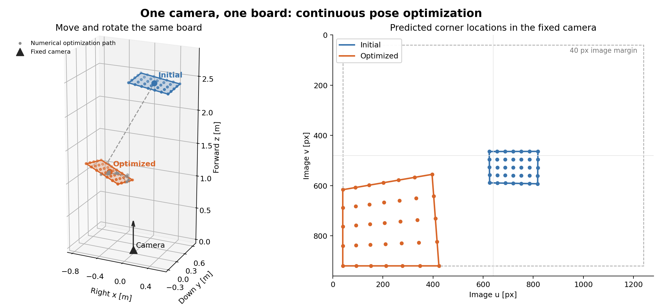
The optimized board is closer, occupies more of the image, and has a different viewing direction and tilt. Together these changes reduce the normalized covariance trace by 98.9%. The optimum reaches the allowed minimum centre depth and the left and bottom image margins. Its largest corner incidence angle is $56.9^\circ$, within the $70^\circ$ limit.
This is a constrained local optimum under the stated model, not a proof of the globally best board pose. In particular, the ideal camera model has no additional penalty for uncertain intrinsics, lens distortion, or peripheral detection errors. Adding those effects, or board-survey uncertainty, can change the optimized pose. The result is not a general instruction to put every calibration board in an image corner.
Board Position in the Camera View During Optimization
The following snapshots select iterations 0, 1, 2, 7, 14, 21, 22, 28, and 35 from the same optimization history. They are intermediate states of one continuous optimization, not separate experiments or candidate layouts used to choose a winner. Read left to right, then top to bottom.
Each panel projects the same board through the fixed camera, with identical image dimensions and pixel axes. The checker pattern spans the known corner grid; its coloured outline and dots show the projected footprint and all 35 corners. The dashed rectangle marks the required 40-pixel image margin. Each title gives the iteration and camera-uncertainty objective $U$.
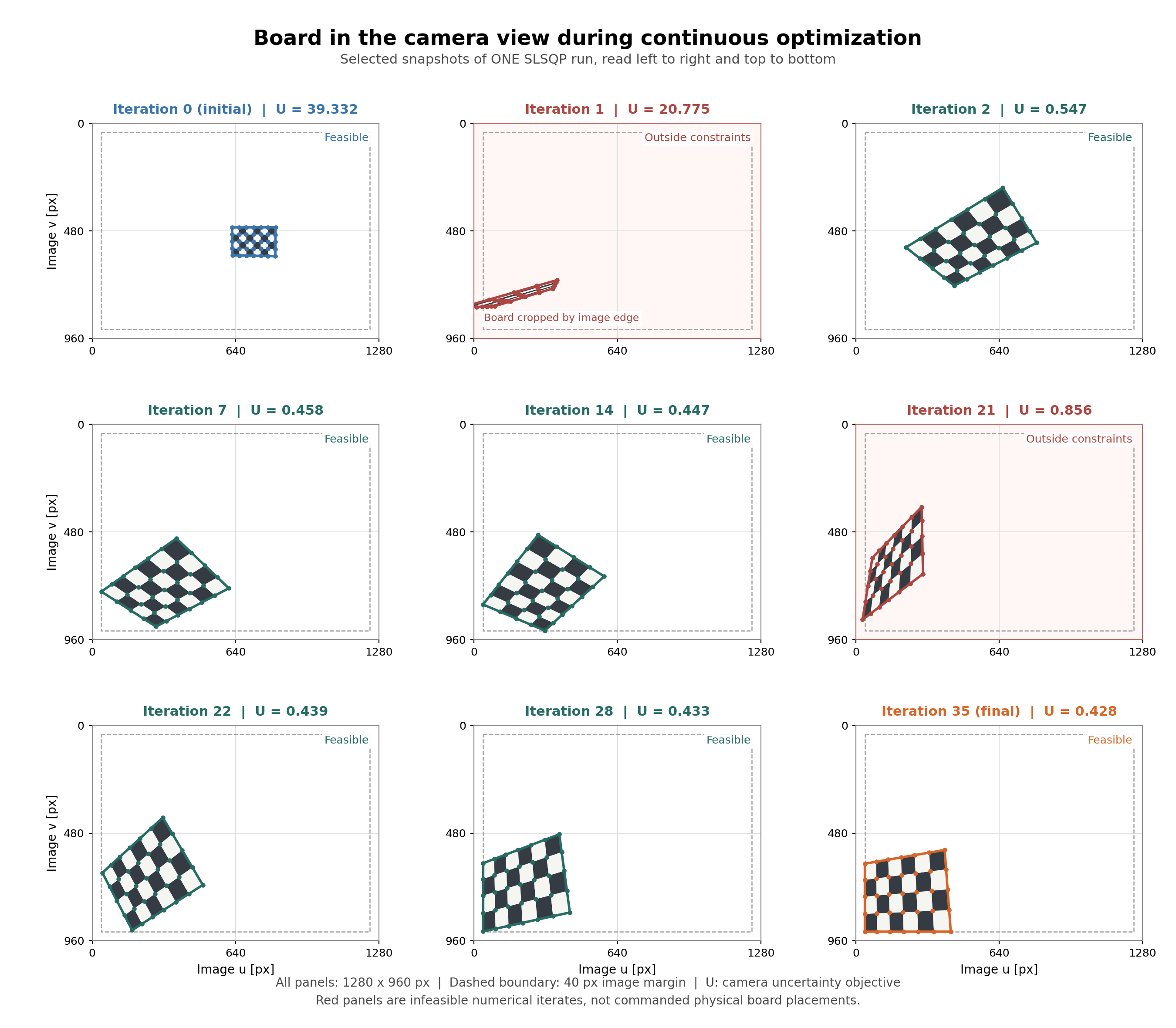
Initially the board appears small, near the image centre. By iteration 2 it is substantially larger; later updates shift and rotate its projection toward the lower-left region. Iterations 1 and 21 violate constraints and are shown explicitly rather than hidden: iteration 1 even puts part of the board outside the image. These are numerical optimizer states, not instructions to physically move the board through those poses. At iteration 35 the projected board satisfies the constraints and touches the allowed left and bottom margins.
The selected-iteration data records the exact six-coordinate board poses, uncertainty scores, and feasibility flags used for this figure. The full optimization history includes every recorded iteration.
Why Not Place the Board Symmetrically at the Image Centre?
A centred board is an intuitive choice, but visual symmetry does not automatically minimize the uncertainty of all six camera-pose parameters. The off-centre result needs a precise interpretation: the centre is competitive, and the lower-left corner is not uniquely optimal.
To check the effect of centring, fix the physical board centre on the optical axis, $x_B=y_B=0$, and continuously optimize the remaining four coordinates:
$$ \underset{z_B,\alpha,\beta,\gamma}{\operatorname{minimize}}\; U(0,0,z_B,\alpha,\beta,\gamma), \qquad (0,0,z_B,\alpha,\beta,\gamma)\in\mathcal S. $$This uses the same objective, noise model, and feasibility constraints as the six-coordinate optimization. SLSQP starts from the previous solution’s depth and orientation, with its lateral position reset to zero. It converges in 16 iterations to a local centred solution with $z_B=1$ m and approximately $(\alpha,\beta,\gamma)=(0^\circ,49.57^\circ,-10.52^\circ)$. Thus, “centred” does not mean “front-facing”: the board centre projects to the principal point, but its orientation remains free.
| Continuously optimized placement | Predicted translation RMS (mm) | Predicted rotation RMS (deg) | Objective $U$ |
|---|---|---|---|
| Board centre constrained to the optical axis | 1.07 | 0.0666 | 0.4893 |
| Off-centre solution shown above | 1.24 | 0.0605 | 0.4277 |
The centred solution actually has better predicted translation precision. The off-centre solution sacrifices some translation precision for better rotation precision, and the chosen $5$ mm / $0.1^\circ$ normalization favors that trade-off. Its objective is only 12.6% lower than this optimized centred solution. The earlier 98.9% reduction is relative to the distant initial pose and combines changes in depth, orientation, and lateral position; it is not a 98.9% advantage of off-centre placement over centred placement.
This is a diagnostic constrained optimization, not a selection among manually prescribed experiments. Both reported solutions are local numerical solutions, not proofs of global optimality.
The geometric reason is that different camera motions can produce similar image motions. For a camera-frame point $(X,Y,Z)$, the unwhitened horizontal pixel coordinate has the following derivatives under the camera-perturbation convention used above:
$$ \frac{\partial u}{\partial t_x}=-\frac{f}{Z}, \qquad \frac{\partial u}{\partial\omega_y}= -f\left(1+\frac{X^2}{Z^2}\right). $$Here $t_x$ and $\omega_y$ refer to camera translation and rotation, not board-design coordinates. For a nearly front-facing board near the image centre, $X/Z$ is small and corner depths are similar. Both a sideways camera translation and a small rotation about the camera’s $y$ axis then produce approximately uniform horizontal image shifts. Their Jacobian columns are nearly proportional, making those camera parameters difficult to distinguish.
Tilting the board introduces depth variation across corners, while moving it off-axis changes the spatial pattern of rotational image motion. Either can help separate the effects of different pose parameters. Symmetry can reduce some parameter correlations, but does not eliminate this translation-rotation coupling. The objective accounts for the joint correlations through $C=(J^\top J)^{-1}$, rather than scoring only the diagonal of $J^\top J$. These are local covariance predictions under the assumed measurement noise, not measured real-camera accuracies; see the Ceres covariance documentation.
Symmetry also does not imply that the minimum must occur at the centre. In this model, reflecting both the board position and orientation horizontally or vertically preserves the score. All four mirrored versions of the off-centre solution were checked: they satisfy the constraints and have the same $U=0.42765855$. The lower-left placement is therefore one member of a symmetry-related set, not a uniquely preferred image region.
For the fixed-axis xyz Euler convention used here, horizontal reflection changes the signs of x, beta, and gamma; vertical reflection changes the signs of y, alpha, and gamma. Applying both gives the fourth pose. Reflecting only the board centre while retaining its original orientation is not this symmetry check.
Finally, the model assumes exact intrinsics, no lens distortion, and an exactly known board pose. Its noise model penalizes grazing incidence but includes no additional penalty for peripheral-image errors. Uncertainty in intrinsic calibration, residual distortion, actual corner-detection quality, and board surveying can change the optimum. The conclusion is a model-specific translation-versus-rotation trade-off, not a general recommendation to move calibration boards to image corners.
Reproduce the Centred-Placement and Symmetry Checks
From the repository root, run the simulation source with NumPy, SciPy, and Matplotlib installed:
python content/posts/2025-02-EOL-calib/simulations/one_camera_one_board_placement.py --centred-checks-only
This command first reruns the original six-coordinate optimization from the stated initial pose. It then fixes the lateral coordinates to zero, initializes depth and orientation from that computed solution, and optimizes the remaining four coordinates. Finally, it constructs and checks all four mirrored off-centre poses. It does not read saved solutions, generate noisy observations, or use Monte Carlo errors to select a placement.
Both optimizations use scaled variables, SciPy’s default numerical derivatives, and a maximum of 200 SLSQP iterations. The objective stopping tolerance ftol is 1e-10 for the original optimization and 1e-11 for the centred diagnostic. The script rejects unsuccessful optimization, final poses violating a nonlinear constraint or coordinate bound beyond a slack tolerance of 1e-7, and failed camera-Jacobian finite-difference checks. For the mirrors, it checks equality of the objective and both predicted RMS errors with relative tolerance 1e-10 and absolute tolerance 1e-12.
The command regenerates these files in the article’s resources/ directory; add --output-dir /tmp/ocob-centred-checks to write elsewhere:
- Centred/off-centre comparison: exact poses, predicted errors, objective values, and iteration counts behind the table above.
- Centred optimization history: the starting pose and every recorded iterate, with both lateral coordinates fixed to zero.
- Mirror-symmetry checks: all four poses, feasibility flags, uncertainty metrics, and score differences from the original pose.
- Reproducibility record: starting poses, variable scales, tolerances, solver outcomes, package versions, and the calculated 12.6% score reduction.
The saved results used Python 3.10.9, NumPy 1.23.5, SciPy 1.10.0, and Matplotlib 3.7.0. Other numerical builds may change the last digits or iteration counts. The accompanying regression tests verify the reported values within numerical tolerances, the translation-versus-rotation trade-off, and the reflected board geometry. The full simulation command below also regenerates these diagnostics before running its separate noisy-fit validation.
Estimate the Camera After Moving the Board
Once the optimized pose is chosen, move and re-survey the board, acquire an image, and estimate the camera pose by minimizing the whitened reprojection loss over $T_C$:
$$ \widehat T_C= \underset{T_C}{\arg\min}\; \frac12\sum_i \left\| \frac{ \pi_K\!\left(R_C^\top[X_i(s^\star)-t_C]\right)-u_i }{\sigma_i(s^\star)} \right\|^2. $$Here $\pi_K$ is pixel projection and $u_i$ is the measured corner. Unlike the outer optimization over $s$, this inner least-squares problem adjusts the camera estimate while holding the surveyed board fixed.
For validation only, the script generates 500 independent noisy images at the initial pose and another 500 at the optimized pose, and refines the camera estimate for each image. These trials are not inputs to placement optimization, and observations from different images are not accumulated. The reported errors are RMS magnitudes of the full three-dimensional translation or rotation error, not average per-axis standard deviations.
| Camera-error metric | Initial pose | Optimized pose |
|---|---|---|
| Predicted translation RMS (mm) | 20.75 | 1.24 |
| Simulated translation RMS (mm) | 20.59 | 1.23 |
| Predicted rotation RMS (deg) | 0.470 | 0.061 |
| Simulated rotation RMS (deg) | 0.467 | 0.060 |
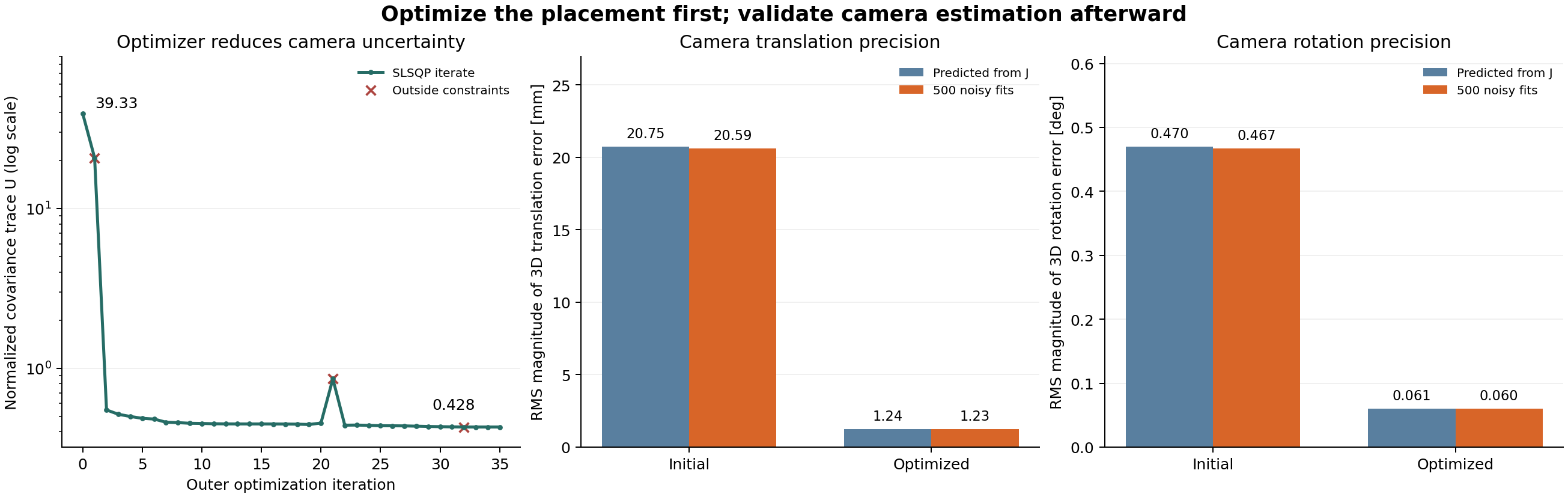
The camera refinements start near the true pose and test the local positive-depth solution branch. They do not test global initialization or planar pose ambiguities; the OpenCV PnP documentation describes methods that can return multiple pose solutions. Likewise, SLSQP’s numerical trajectory is not a collision-checked robot trajectory.
The reproducible simulation source requires NumPy, SciPy, and Matplotlib:
python content/posts/2025-02-EOL-calib/simulations/one_camera_one_board_placement.py
The script checks the camera Jacobian against finite differences and saves the optimization history, placement and uncertainty summary, and individual noisy-fit errors. The example’s key sequence is: predict camera uncertainty, optimize the board pose, then collect measurements and estimate the camera.
4.2 Two Cameras, One Board: Corner Refinement and Calibration
This two-camera, one-board experiment checks board-survey refinement, image-corner localization, and pose estimation at a fixed board placement; it is not a second placement-search algorithm. The geometric preprocessing is derived in Appendix A, and the two-camera objective is written explicitly in Appendix D.
We construct an 8x8 chessboard with 1 m squares. We set the the origin as the center of the board. We place the board in the world coordinate with extrinsic:
$$\begin{pmatrix} 1 & 0 & 0 & 0 \\ 0 & 1 & 0 & 0 \\ 0 & 0 & 1 & 8 \\ 0 & 0 & 0 & 1 \end{pmatrix} $$which means the normal of the board plane is $[0, 0, 1]^\top$.
We add Gaussian noise on the corners coordinates with noise zero mean and $0.005$ standard deviation.
With the noisy corners’ coordinates, we can get the optimized board’s extrinsic using the rigid board-fit procedure in Appendix A. The optimized normal is $[1.38*10^{-3}, -2.16*10^{-5}, 9.999*10^{-1}]^\top$. That is already very close the ground truth.
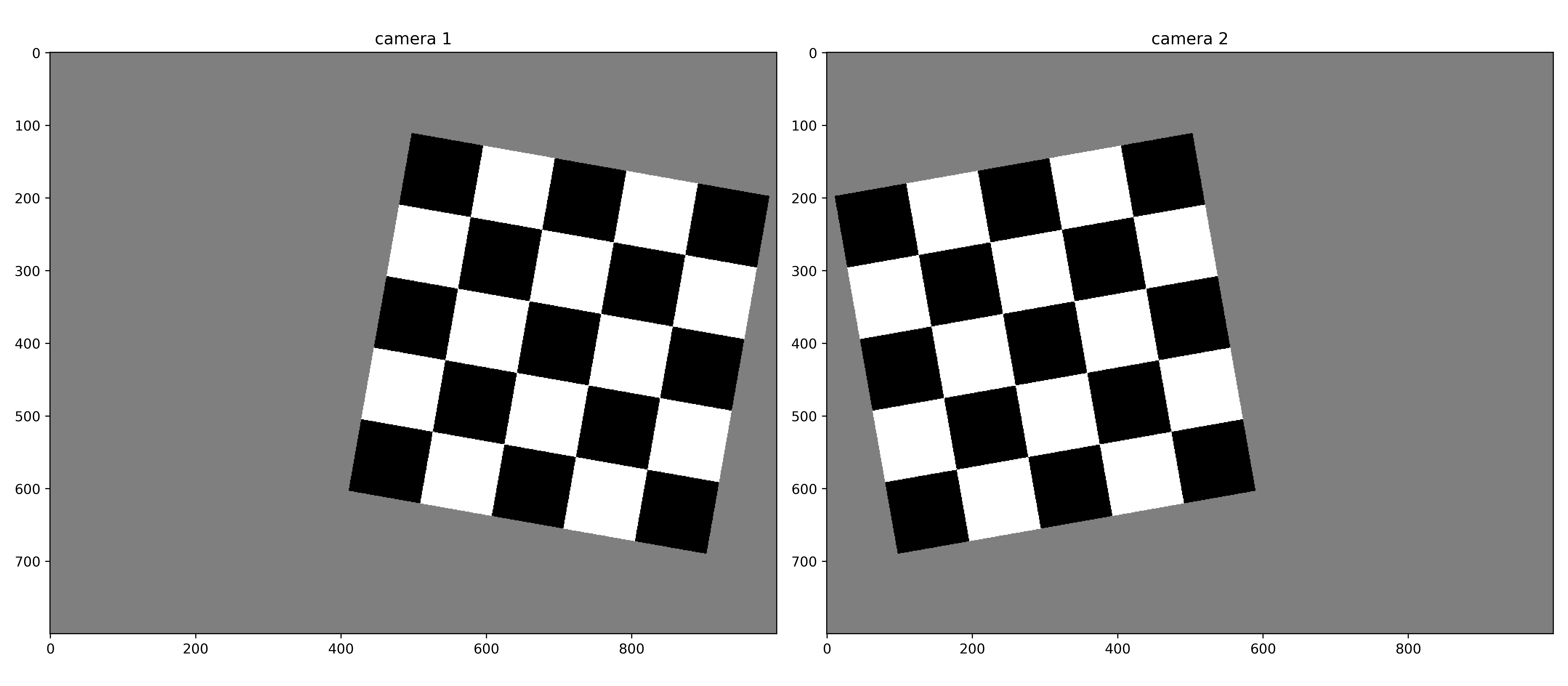
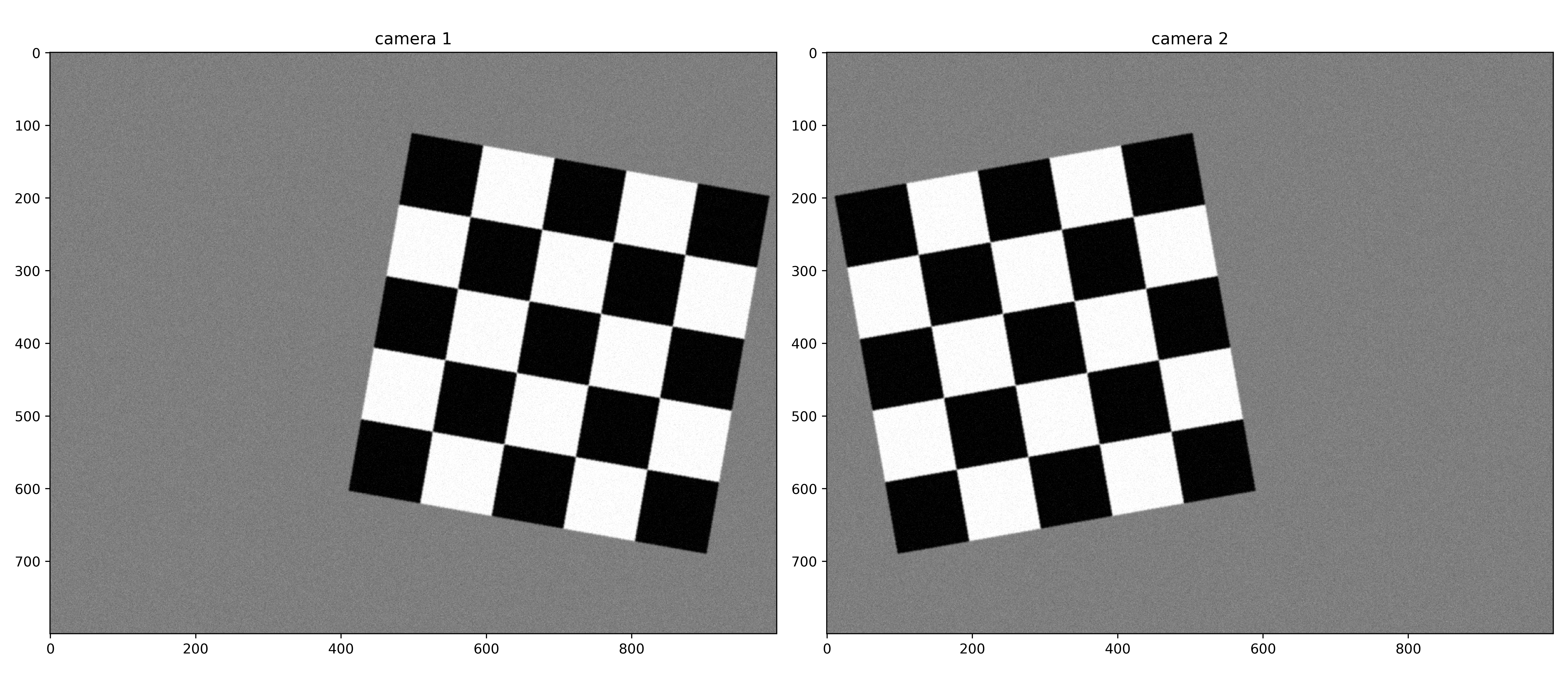
Then we simulate two cameras with the same intrinsic matrix: $f_x =800$, $c_x = 500$, $f_y = 800$, $c_y=400$, and $H=800$, $W=1000$. We rotate the first camera along the z-axis $10$ degrees and the second $-10$ degrees, and translate the first camera along the x-axis $2$ meters and the second $-2$ meters. Then the images of the chessboard in the two cameras are shown in the figure below.
Then, we apply Gaussian blur on the observed images and add Gaussian noise on them. The new images are shown in the figure below.
After that, we use opencv “findChessboardCorners” and find the rough corners and then use “cornerSubPix” to refine the corners’ coordinates. The refined corners are shown in the figure below.
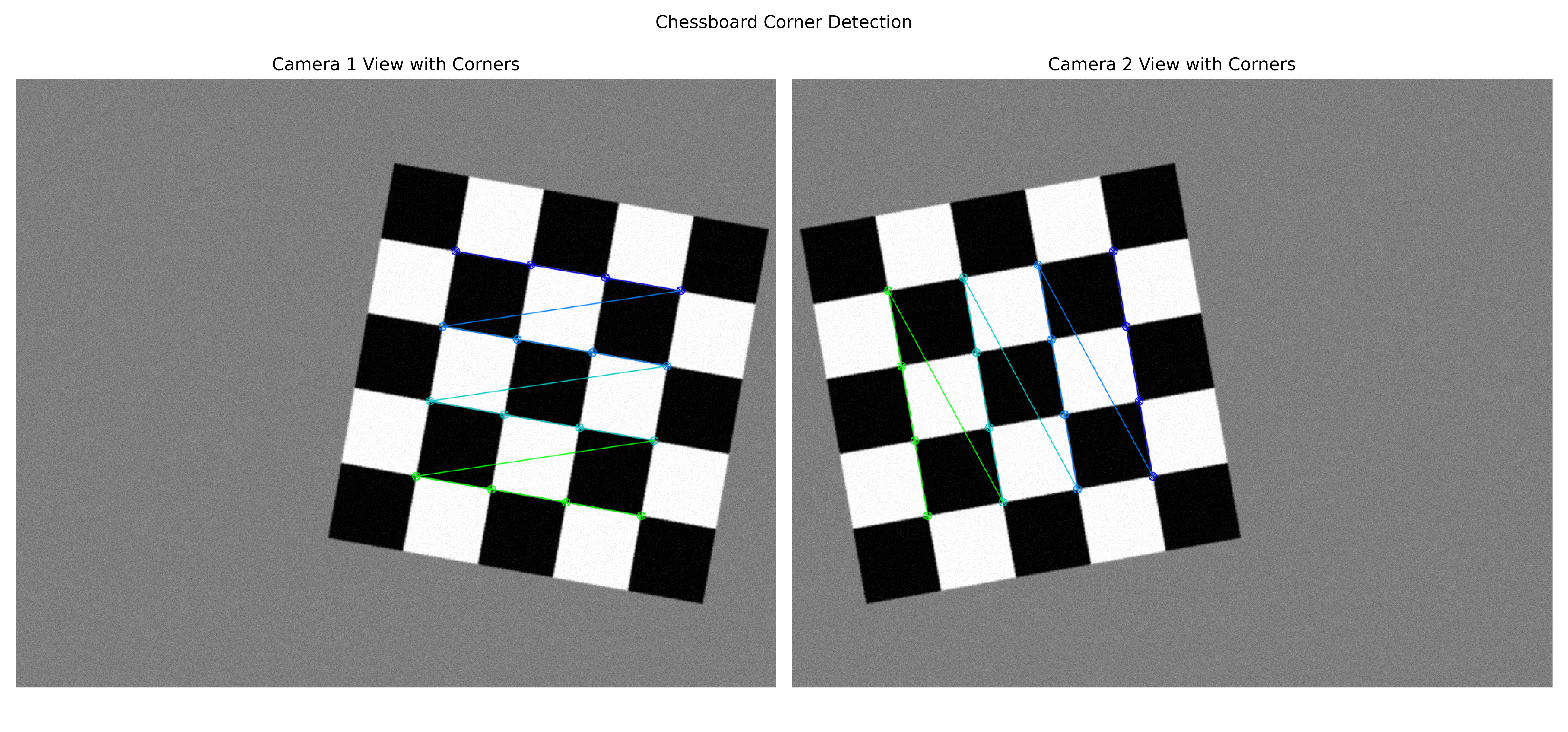
Pay attention to the sequence of the detected corners. (The detected corners start from the blue one and end with the green one in the above figure.) Rearrange the detected corners according to the refined chessboard corners. Using the “solvePnP” function with method “SQPNP”, which is a global optimization method, we can find the estimated extrinsic of the two cameras. We record the errors of the estimation using the original measurements of the chessboard corners and the refined ones.
| Camera | Corners | Rotation Error (degrees) | Translation Error (meters) |
|---|---|---|---|
| Camera 1 | Original | 0.260 | 0.0372 |
| Camera 1 | Refined | 0.0732 | 0.0117 |
| Camera 2 | Original | 0.247 | 0.0318 |
| Camera 2 | Refined | 0.0750 | 0.0118 |
The translation error is the norm of the difference between the estimated and the ground truth translation. The rotation error is
$$ \theta= \left\| \operatorname{Log}_{SO(3)} \left( \mathbf{R}_{\rm gt}^{\top}\mathbf{R}_{\rm est} \right) \right\|_2, $$converted from radians to degrees.
As shown in the table, the refined measurements result in lower errors for both rotation and translation, demonstrating the effectiveness of the corner refinement process.
In the final step, we do jointly optimization. We warp the image in camera 1 with parameters before and after jointly optimization. The results are shown in the figure below.
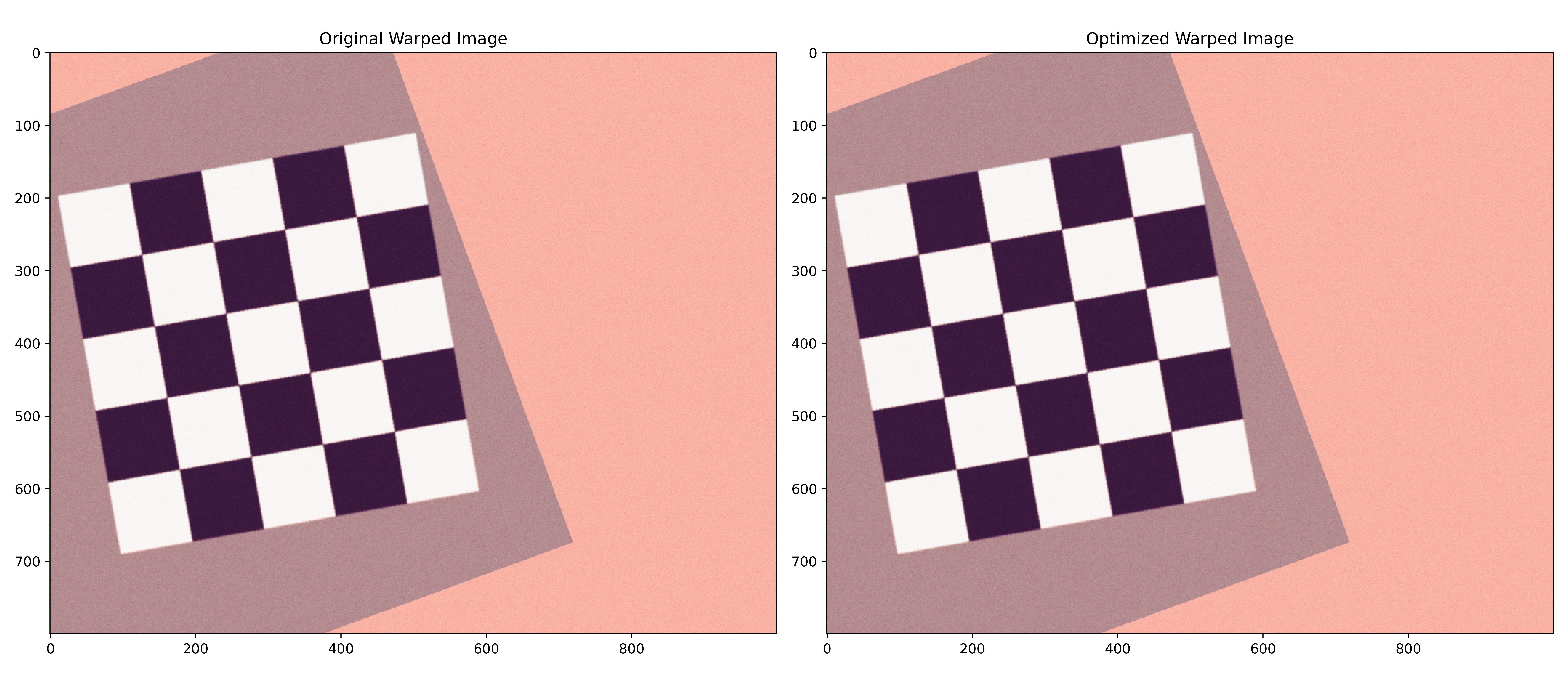
In the above figure, we can hardly tell which one is better. The translation error is $0.0298$ and $0.0257$ meters for camera 1 and camera 2 respectively. The rotation error is $0.204$ and $0.199$ degrees for camera 1 and camera 2 respectively. That is expected increased error for single camera calibration however more consistent for the two cameras.
Detect Corners on the Warped Image
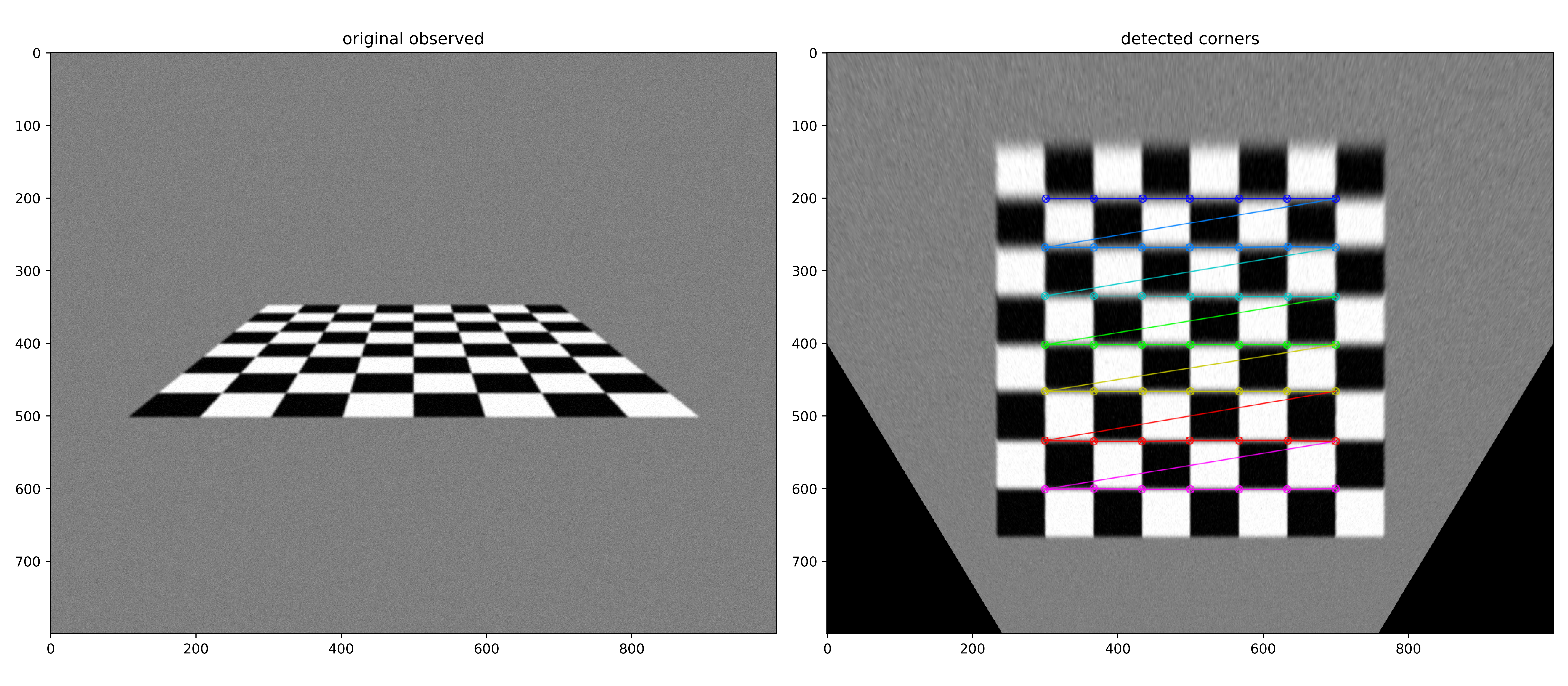
Corner detection often becomes challenging on original images due to severe distortion or extreme viewing angles. To address this limitation, we can create a virtual camera with an optimized viewpoint. By warping the original image onto this virtual camera’s image plane, we can simulate a more frontal view of the chessboard. This transformation adjusts the perspective so that the chessboard appears as if viewed head-on, significantly improving corner detection reliability. We can then accurately detect the corners on this warped image rather than struggling with the difficult perspective of the original.
The figure below illustrates this approach. On the left is the original image where the severe viewing angle prevents the standard algorithm from successfully detecting the corners. On the right is the perspective-corrected warped image, where we can successfully identify and locate all corners.
4.3 Two Cameras, Two Boards: Uncertain Boards and Discrete Placement
Building on the one-camera placement optimization in Section 4.1, consider a calibration station with two cameras and two physical calibration boards. Here the lower level estimates both camera poses and both uncertain board poses from noisy image corners and noisy surveyed board corners. This separate experiment uses a discrete candidate set to illustrate several upper-level search strategies; Section 4.1 demonstrates direct continuous board-pose optimization from one starting pose.
The experiment is generated by:
python chess-board-simulate/two_camera_two_board_placement.py
The two cameras are fixed and look into a shared workspace. Each board has a $7\times5$ marker grid with $0.12$ m spacing. Candidate board poses are sampled over position, height, yaw offset, and tilt. A candidate is feasible only if both cameras see at least 20 corners, the projected corners are inside the image margin, the projected marker size is large enough, and the board is not too grazing.
Noise Model
The simulated image noise follows the placement-dependent idea from the bilevel formulation. For each visible corner, the pixel standard deviation is
$$ \sigma_{u,cp} = \operatorname{clip} \left( 0.28 \left[ 1 + 0.35\left(\frac{18}{a_{cp}}\right)^2 + 0.16\left(\frac{1}{\max(\iota_{cp},0.10)}-1\right) + 0.30\rho_{cp}^2 \right], 0.25, 3.5 \right)\ \mathrm{px}. $$Here $a_{cp}$ is the projected marker size in pixels, $\iota_{cp}$ is the incidence between the board normal and the camera ray, and $\rho_{cp}$ is normalized distance from the image center. This makes small, oblique, or edge-of-image corners noisier. Surveyed world marker positions use $\sigma_z=2.5$ mm.
Upper-Level Solvers
For each feasible candidate board pose $g$, the script predicts visibility and computes the Schur-marginalized camera-pose information contribution $\Delta\Lambda_g$. For a selected two-board set $\mathcal A=\{g_1,g_2\}$, the A-optimal score is
$$ U(\mathcal A) = \operatorname{tr} \left[ D \left( \sum_{g\in\mathcal A}\Delta\Lambda_g \right)^{-1} D^\top \right]. $$The simulation compares four placement strategies:
- Manual initial: two nearby, front-workspace boards.
- Greedy next-best: choose the first board with the best single-board score, then choose the second board that gives the best updated two-board score.
- Simulated annealing: start from the manual pair, randomly replace one board at a time, and accept or reject moves using a decreasing temperature.
- Exhaustive optimum: enumerate all valid two-board pairs in the discrete candidate set and choose the pair with the lowest A-optimal trace.
This mirrors the reference strategies in the placement-guidance literature: sample a feasible pose set, reject degenerate candidates, score by parameter uncertainty rather than residual alone, and use either direct search, sequential next-best selection, or simulated annealing to search the pose space.
The feasible candidate set and selected layouts are:
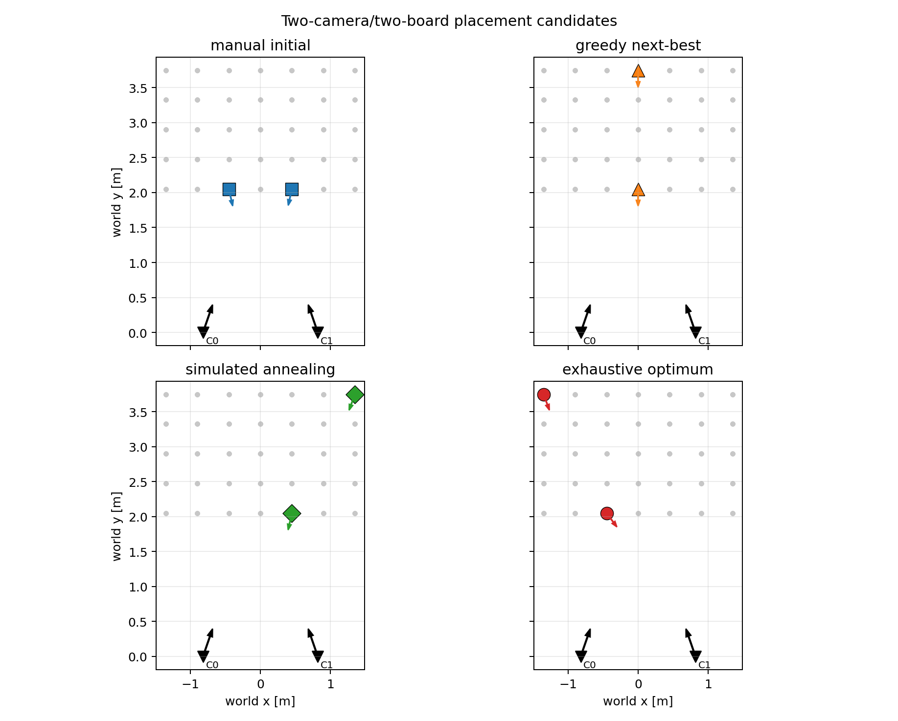
The single-board candidate score map is:
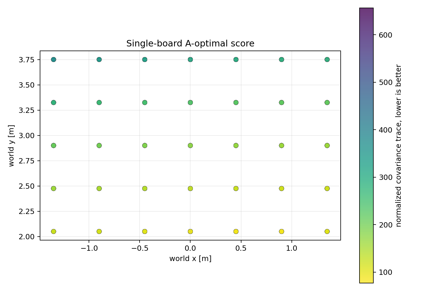
The selected board placements are:
| Layout | Slot | Candidate | x (m) | y (m) | z (m) | Yaw Offset (deg) | Tilt (deg) | Predicted Trace |
|---|---|---|---|---|---|---|---|---|
| manual initial | 0 | P123 | -0.45 | 2.05 | 0.92 | 0.00 | 12.00 | 23.49 |
| manual initial | 1 | P242 | 0.45 | 2.05 | 0.92 | 0.00 | -12.00 | 23.49 |
| greedy next-best | 0 | P189 | 0.00 | 2.05 | 1.18 | 0.00 | 12.00 | 5.97 |
| greedy next-best | 1 | P236 | 0.00 | 3.75 | 1.18 | 0.00 | -12.00 | 5.97 |
| simulated annealing | 0 | P248 | 0.45 | 2.05 | 1.18 | 0.00 | -12.00 | 5.82 |
| simulated annealing | 1 | P417 | 1.35 | 3.75 | 1.18 | 0.00 | 12.00 | 5.82 |
| exhaustive optimum | 0 | P050 | -1.35 | 3.75 | 0.92 | 0.00 | -12.00 | 5.73 |
| exhaustive optimum | 1 | P130 | -0.45 | 2.05 | 1.18 | 24.00 | -12.00 | 5.73 |
The optimized placements are not chosen by reprojection residual. They spread the two boards in depth, lateral position, height, and tilt so that the camera-pose Jacobians span stronger independent directions.
Noisy Lower-Level Validation
After selecting the placements, each layout is validated by 24 Monte Carlo trials. Each trial re-samples image noise and surveyed board-corner noise, then solves the lower-level bundle-adjustment problem from perturbed initial camera poses.
| Layout | Observations | Pixel RMSE (px) | Predicted Trace | Trace / Best | Pred. Rot. Std. (deg) | Pred. Trans. Std. (mm) | MC Rot. Error (deg) | MC Rot. Std. | MC Trans. Error (mm) | MC Trans. Std. |
|---|---|---|---|---|---|---|---|---|---|---|
| manual initial | 140 | 0.4215 | 23.4863 | 4.0971 | 0.0931 | 3.3369 | 0.1284 | 0.0421 | 4.9256 | 1.5130 |
| greedy next-best | 140 | 0.4461 | 5.9744 | 1.0422 | 0.0479 | 1.3878 | 0.0522 | 0.0170 | 2.1414 | 0.5751 |
| simulated annealing | 140 | 0.4589 | 5.8206 | 1.0154 | 0.0472 | 1.3992 | 0.0501 | 0.0188 | 2.1440 | 0.5569 |
| exhaustive optimum | 140 | 0.4624 | 5.7324 | 1.0000 | 0.0468 | 1.4088 | 0.0490 | 0.0181 | 2.2678 | 0.6703 |
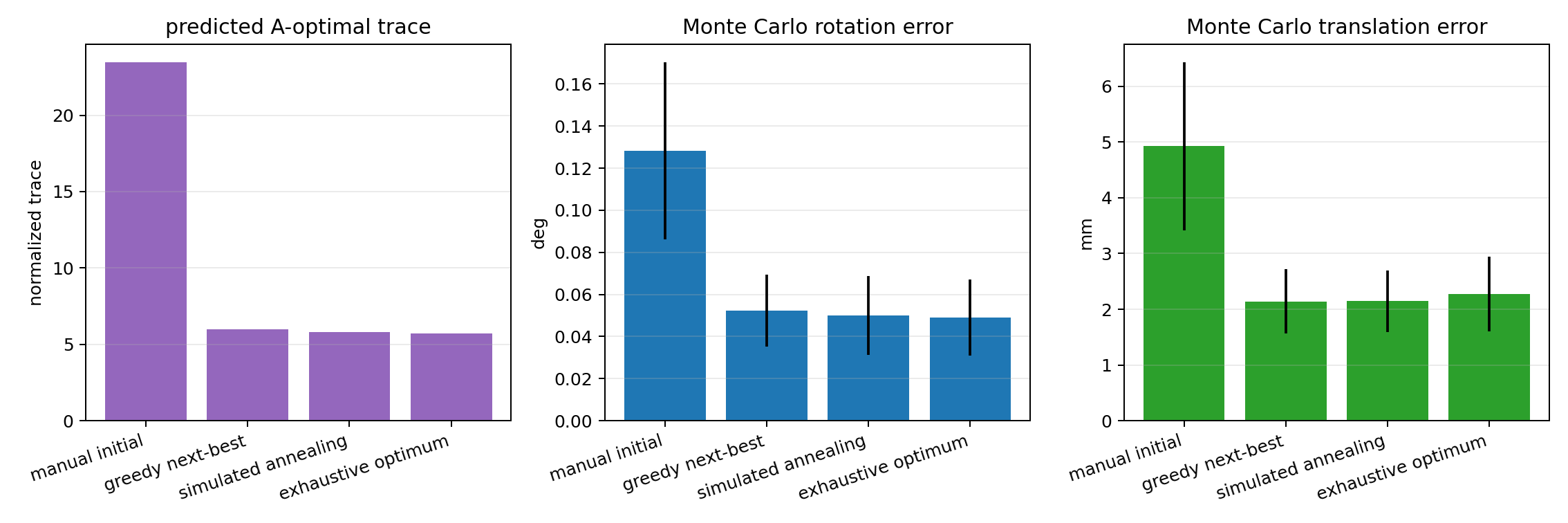
The important observation is that the manual layout has the lowest pixel RMSE, but the worst camera-pose accuracy. It fits its own observations well while leaving weak pose directions. The optimized layouts increase the pixel RMSE slightly, because the views are more oblique and noisy, but they reduce the predicted camera covariance trace by about $4\times$ and reduce the Monte Carlo camera-pose error from $0.128^\circ$ and $4.93$ mm to about $0.05^\circ$ and $2.1$-$2.3$ mm.
This illustrates the same bilevel principle: the upper level should not optimize expected residual. It should optimize the information geometry of the lower-level calibration problem.
4.4 Multi-Board and Multi-Camera Calibration
The simulation code for the two-camera chessboard experiment in Section 4.2 is in livey/chess-board-simulate. A companion script, multi_board_multi_camera.py, now runs a scaling study for the multi-board and multi-camera formulation in this post.
The synthetic scenarios contain:
- Four to eight calibrated cameras with known intrinsics.
- Six to twenty-four target boards, each carrying a $7\times5$ grid of marker points.
- Noisy camera-point observations $u_{cp}$.
- Noisy surveyed world measurements of board marker points.
- Partial visibility: each camera sees only a subset of boards and marker points.
This section reports centralized bundle adjustment, which directly solves (P) over the camera and board poses. The solver-comparison tables, ADMM convergence plots, and communication results are collected in the independent ADMM comparison.
The simulation can be reproduced with:
cd chess-board-simulate
python multi_board_multi_camera.py
The script writes figures and CSV tables into logs/multi_board_multi_camera/. The detailed figures below use the largest case, with eight cameras and twenty-four boards. The scaling tables compare all scenarios from the same deterministic run.
Problem Size
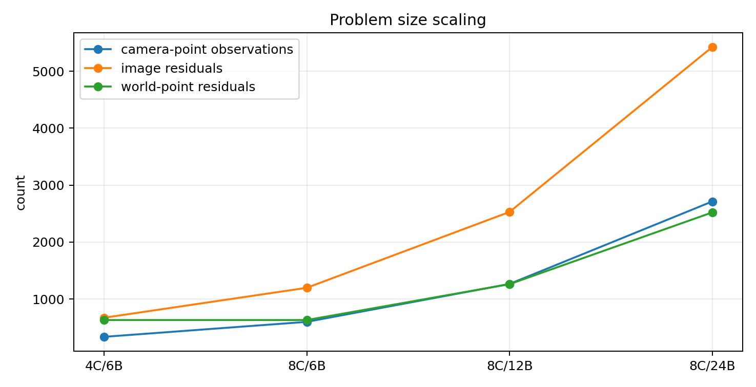
The sweep changes the number of camera poses, board poses, observed camera-point edges, and surveyed board points while keeping the same formulation.
| Scenario | Cameras | Boards | Points per Board | Camera-Board Pairs | Camera-Point Observations | Pose Variables | Image Residuals | World-Point Residuals |
|---|---|---|---|---|---|---|---|---|
| 4_cameras_6_boards | 4 | 6 | 35 | 10 | 335 | 60 | 670 | 630 |
| 8_cameras_6_boards | 8 | 6 | 35 | 18 | 598 | 84 | 1196 | 630 |
| 8_cameras_12_boards | 8 | 12 | 35 | 38 | 1264 | 120 | 2528 | 1260 |
| 8_cameras_24_boards | 8 | 24 | 35 | 82 | 2712 | 192 | 5424 | 2520 |
Simulated Observation Graph
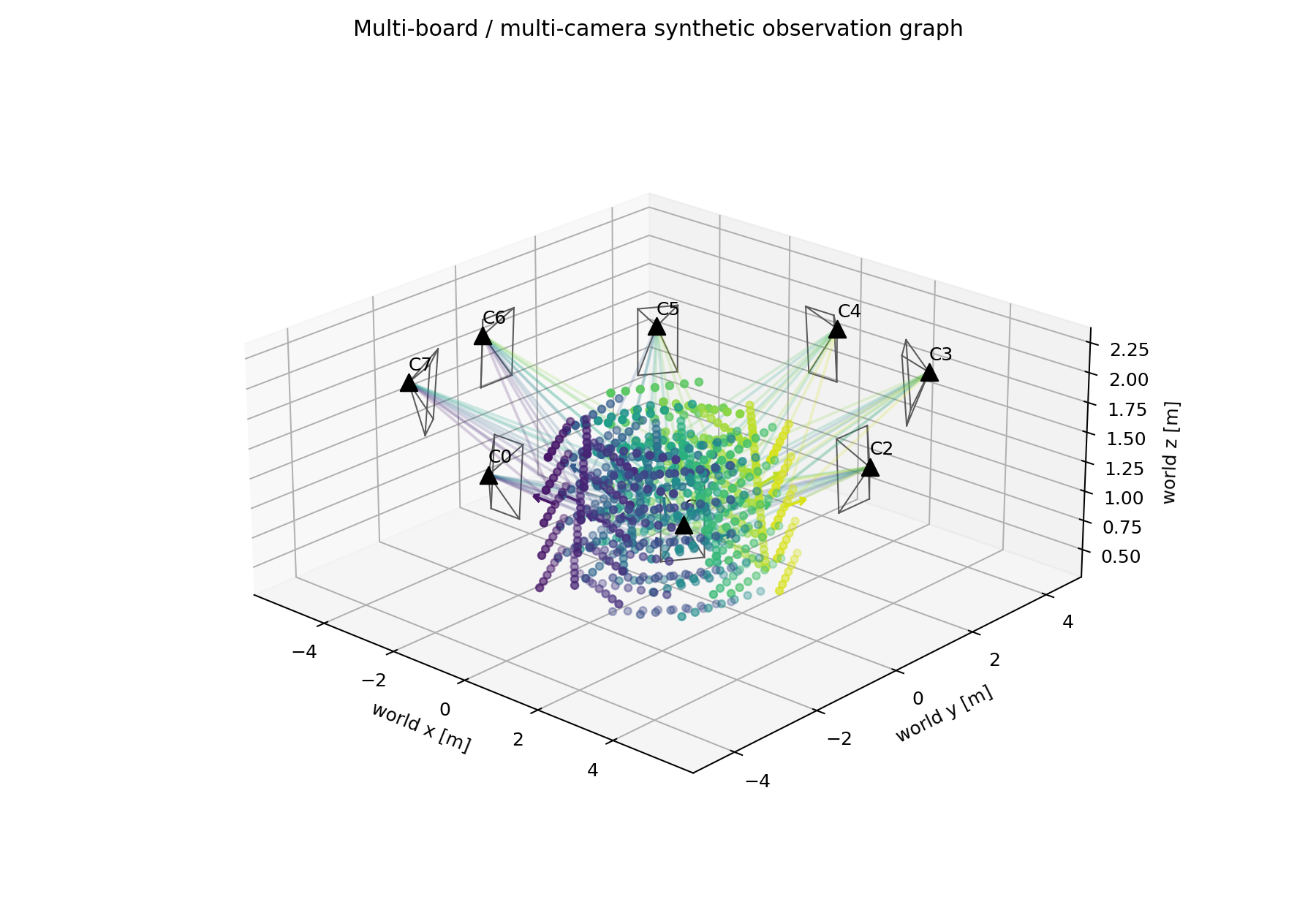
The detailed scene has eight cameras arranged around twenty-four calibration boards. The colored board points are the physical marker locations. The faint lines indicate observed camera-board connections.
The visibility matrix shows how many marker points each camera observes on each board.
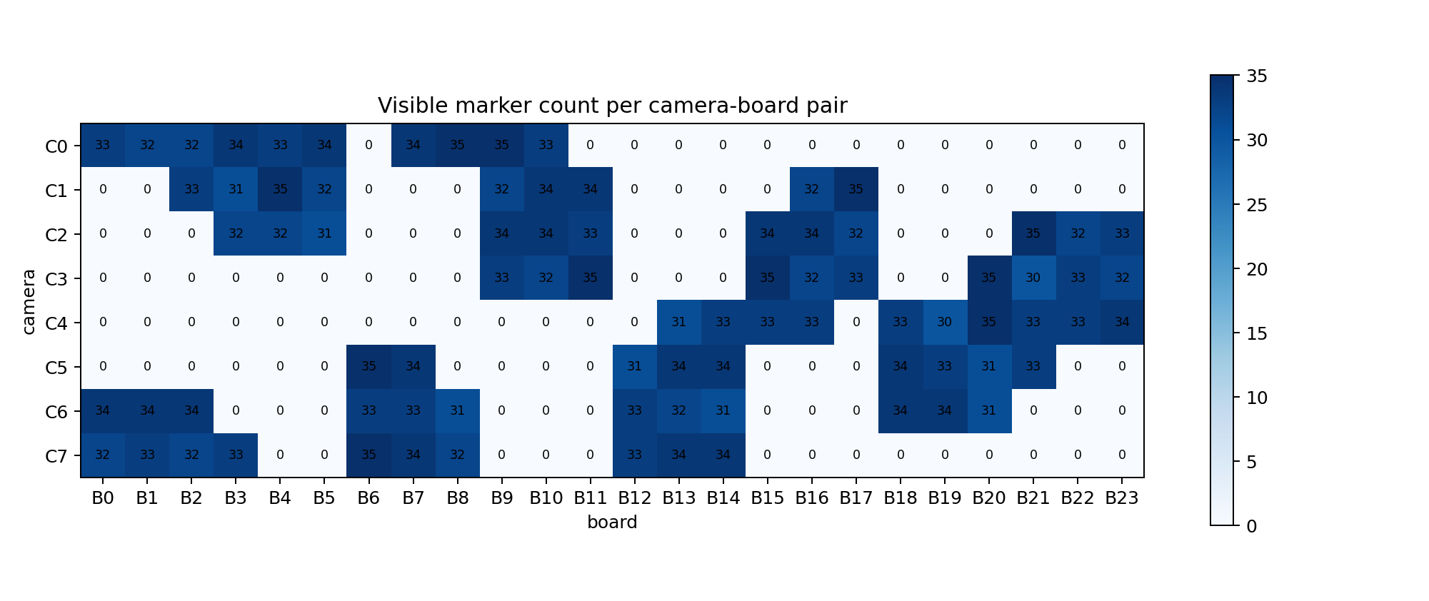
This is intentionally not a complete bipartite graph. In the 8-camera, 24-board case, only 82 of the 192 possible camera-board pairs are visible. The coupling comes from shared boards and world-frame board priors, not from every camera seeing every board. The full $8\times24$ visibility matrix is written to resources/mbmc_visibility_counts.csv.
Image Observations and Reprojection Residuals
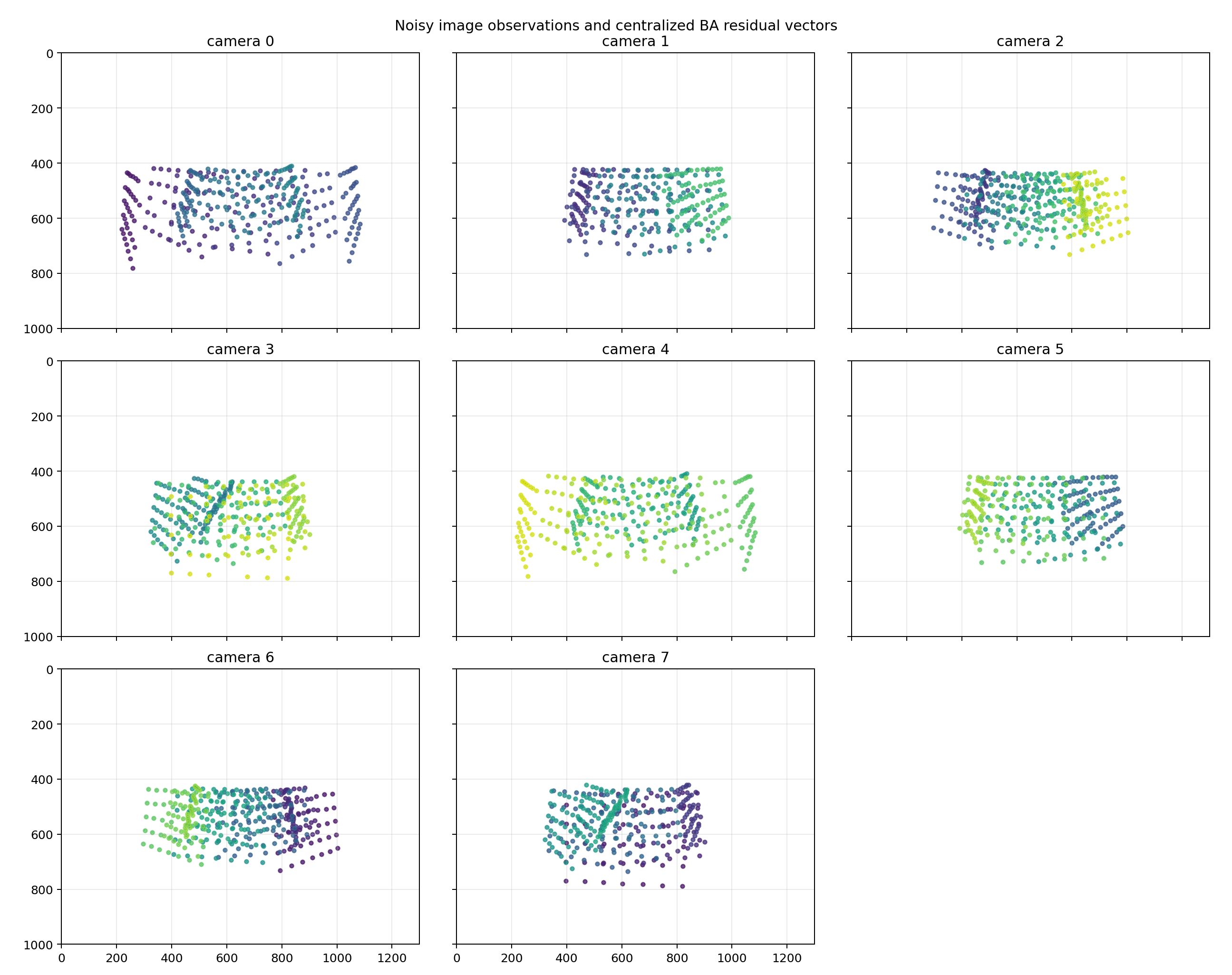
The next figure shows the noisy image observations in each camera. The small black residual vectors connect the measured points to the centralized BA predictions.
Bundle Adjustment Results
For the 8-camera, 24-board case, the initialization perturbs camera poses by several degrees and tens of centimeters, while board poses are initialized from noisy surveyed world marker measurements. Centralized BA reduces reprojection error from 63.0991 px to 1.0486 px.
| Method | Reprojection RMSE (px) | Mean Camera Rot. Error (deg) | Mean Camera Trans. Error (m) | Mean Board Rot. Error (deg) | Mean Board Trans. Error (m) |
|---|---|---|---|---|---|
| Initial | 63.0991 | 4.8642 | 0.2125 | 0.3949 | 0.0032 |
| Centralized BA | 1.0486 | 0.0582 | 0.0036 | 0.1007 | 0.0012 |
The sparse nonlinear least-squares solve takes 1.4180 s and 11 outer iterations in this Python implementation. These are implementation timings for this experiment.
The board error is already small at initialization because the boards are directly anchored by surveyed world points. The camera error drops much more strongly because the image residuals provide most of the camera-pose information. The full per-camera and per-board error tables are written to resources/mbmc_camera_pose_errors.csv, resources/mbmc_board_pose_errors.csv, resources/mbmc_scaling_camera_pose_errors.csv, and resources/mbmc_scaling_board_pose_errors.csv.
Bundle Adjustment Scaling
Centralized BA uses a sparse Jacobian: each image residual touches one camera pose and one board pose. The following results show its accuracy and runtime as the calibration graph grows.
| Scenario | Observations | Central RMSE (px) | Central Runtime (s) |
|---|---|---|---|
| 4_cameras_6_boards | 335 | 1.0046 | 0.1684 |
| 8_cameras_6_boards | 598 | 1.0322 | 0.4938 |
| 8_cameras_12_boards | 1264 | 1.0395 | 1.4527 |
| 8_cameras_24_boards | 2712 | 1.0486 | 1.4180 |
The timings are from the serial Python reference implementation. Reprojection RMSE remains near the pixel noise floor across the four scenarios. The full comparison with the distributed solvers is in the independent comparison.
Board-Placement Guidance Experiment
The same script also runs a next-board-placement experiment. Starting from the solved 8_cameras_6_boards case, it computes the current marginalized camera-pose information from the centralized BA Jacobian. It then generates feasible candidate poses for one additional board, predicts the visible image measurements for each candidate, appends the candidate’s expected Jacobian information, marginalizes the candidate board pose with the Schur complement, and scores the candidate by normalized camera covariance reduction.
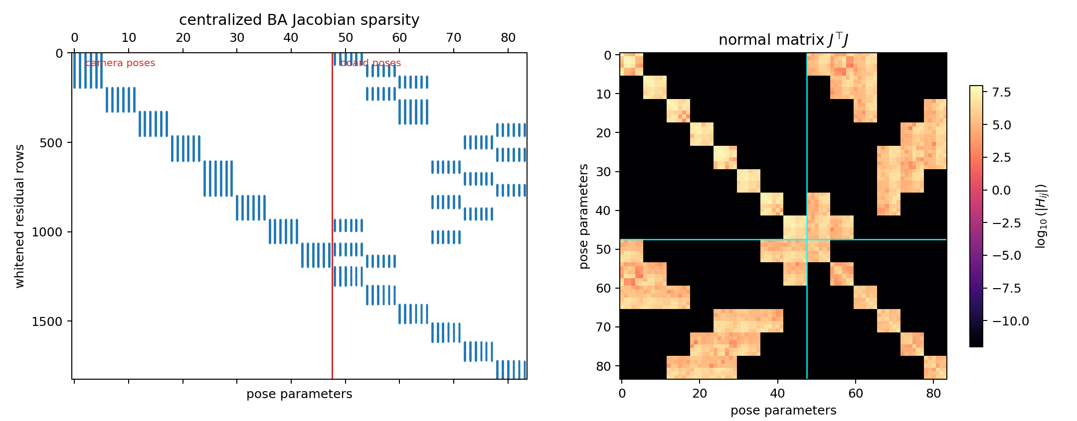
The first diagnostic is the actual optimization matrix. The left plot below is the sparsity pattern of the whitened Jacobian $J$ for the current centralized BA problem. Each reprojection row touches one camera pose and one board pose. Each surveyed world-point row touches only one board pose. The right plot is the Gauss-Newton normal matrix $H_{\mathrm{GN}}=J^\top J$, not the full exact Hessian. This is intentional: near the solved calibration state, and especially for zero-expected-residual candidate measurements, $J^\top J$ is the local curvature/information matrix that determines pose covariance. Its camera-board off-diagonal blocks are exactly the couplings that later become camera-camera information after board poses are marginalized.
The best candidate is not selected by the expected residual value; the expected residual is zero for all candidates. It is selected by the curvature that the candidate observations add to the camera-pose variables.
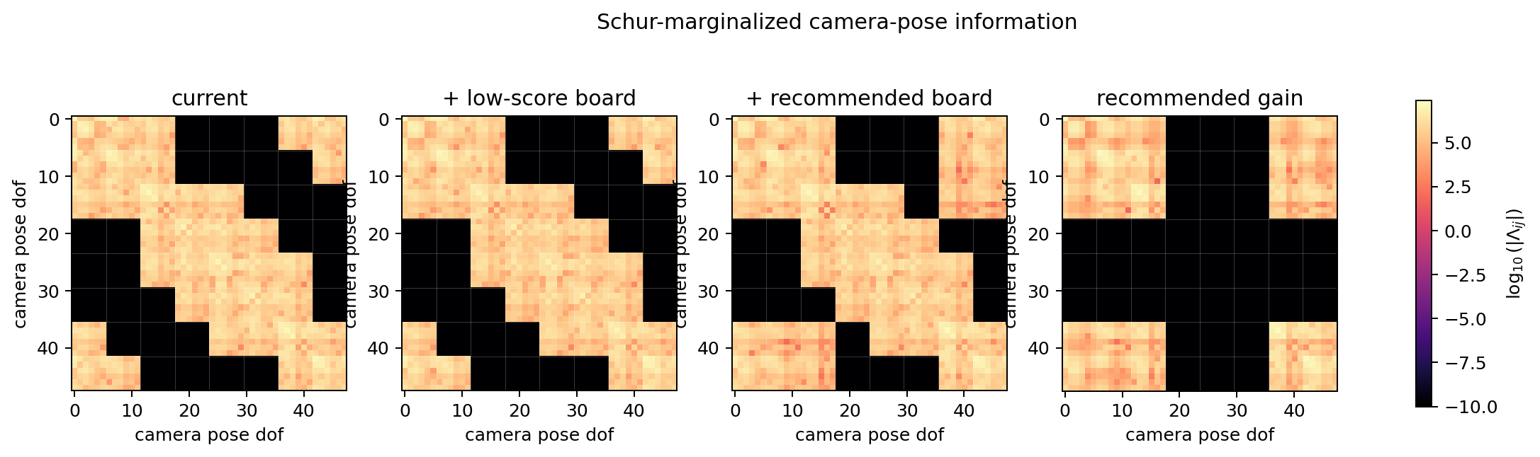
For each candidate board pose, the script computes the candidate’s predicted normal matrix contribution, marginalizes the candidate board pose, and adds the resulting camera-pose information to the current $\Lambda_C$. The next figure shows $\Lambda_C$ before adding a board, after adding the low-score feasible board, after adding the recommended board, and the information gain from the recommended board alone. Each $6\times6$ diagonal block is one camera pose. Off-diagonal blocks indicate camera-camera coupling induced by shared board observations.
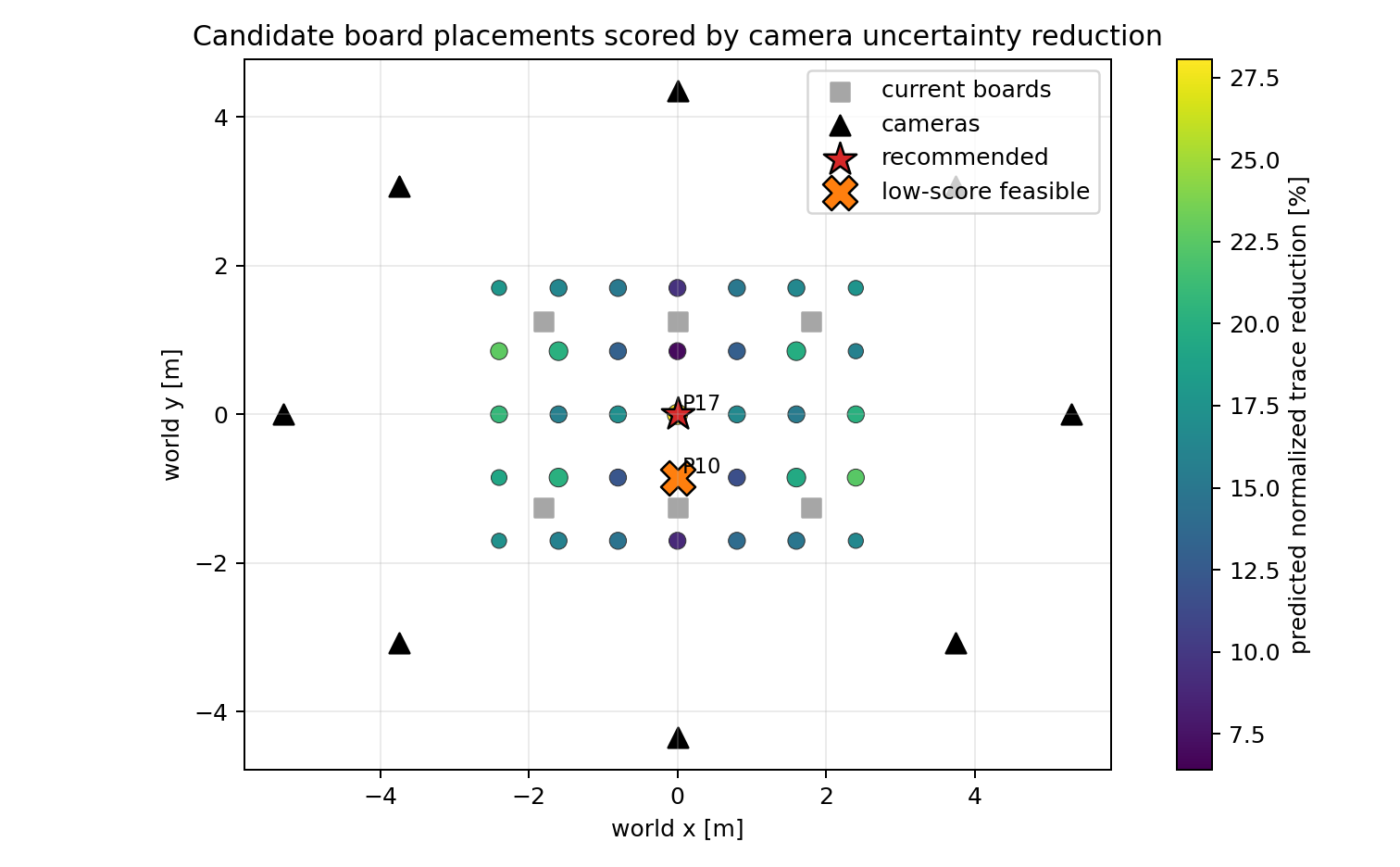
The candidate map below shows all feasible candidate board centers. Color is predicted normalized camera covariance reduction, and marker size increases with the number of predicted marker observations.
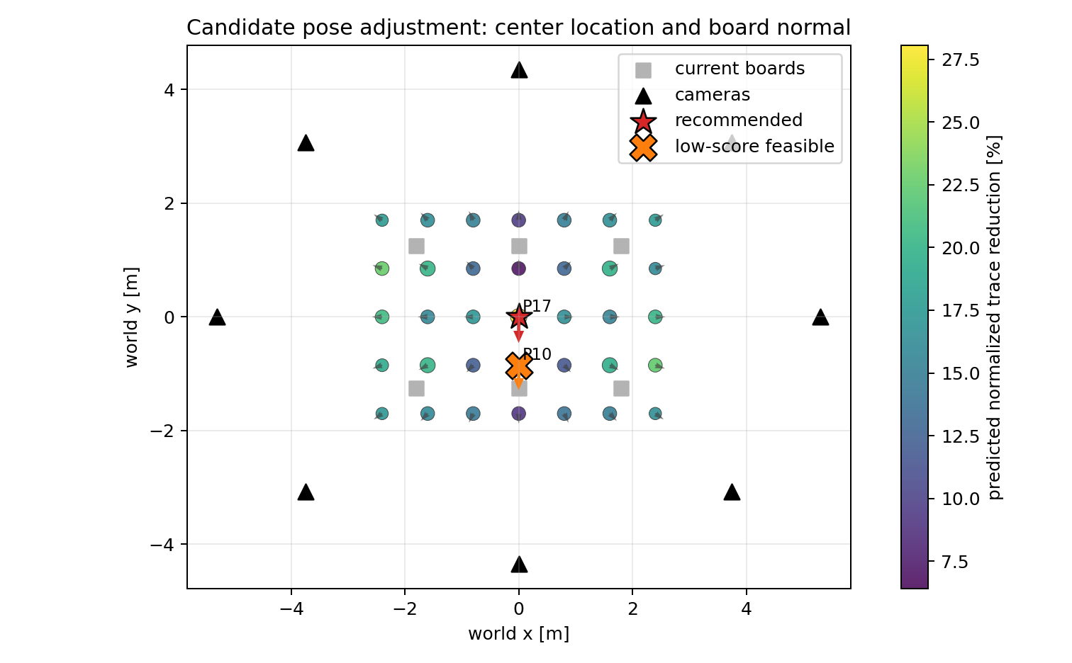
Board placement is not only a center position; it is a pose. The arrows in the next plot show the horizontal component of the board normal. In this experiment, candidate normals are generated to face outward toward the surrounding cameras, and the optimizer selects among these full poses.
The selected candidates are:
| Strategy | Candidate | Position $(x,y,z)$ m | Board Normal | Visible Cameras | Marker Observations | Predicted Trace | Predicted Reduction | Predicted Rot. Std. (deg) | Predicted Trans. Std. (mm) |
|---|---|---|---|---|---|---|---|---|---|
| Recommended | P17 | $(0.00,0.00,1.02)$ | $(0.0000,-0.9348,0.3552)$ | 5 | 175 | 22.5875 | 28.0625% | 0.0651 | 3.5197 |
| Low-score feasible | P10 | $(0.00,-0.85,0.92)$ | $(0.0000,-0.8956,0.4449)$ | 3 | 105 | 29.3866 | 6.4082% | 0.0758 | 3.9703 |
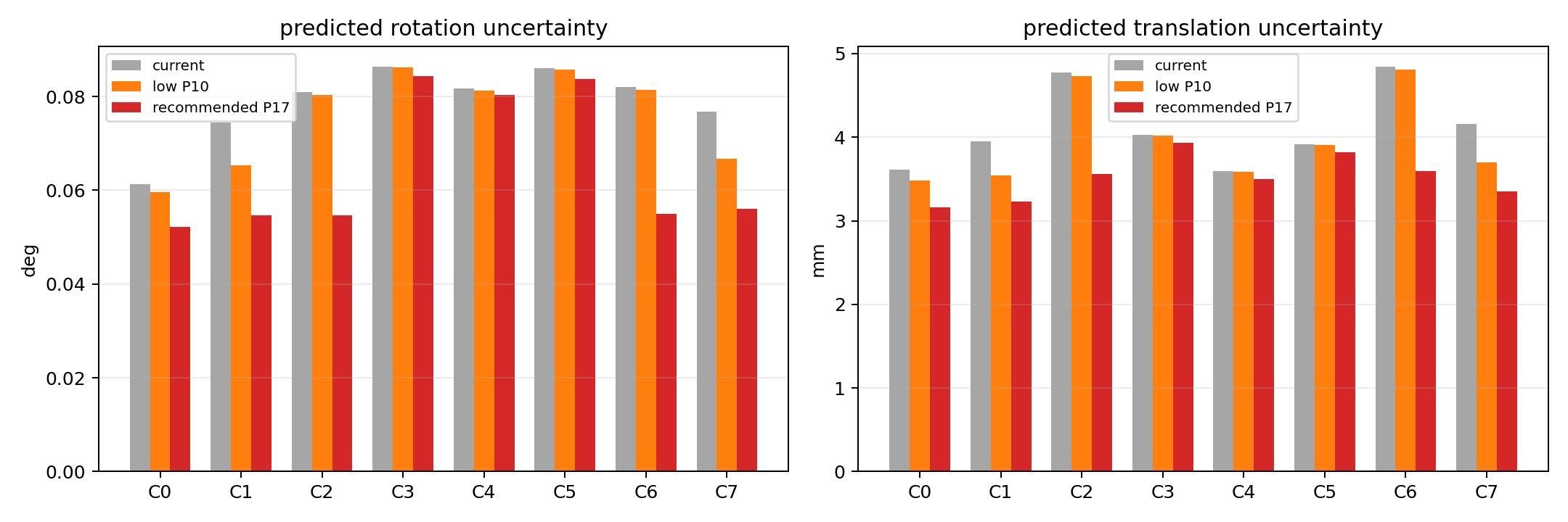
In this current calibration state, the optimizer prefers P17 because it is visible from five cameras and lies in an overlap region. It contributes information to more camera-pose blocks and creates stronger camera-to-camera coupling through one physical board. P10 is still feasible, but its information is more local and therefore reduces the marginalized camera uncertainty much less.
The per-camera uncertainty plot shows where that improvement goes. P17 reduces both rotation and translation uncertainty for more cameras than P10, especially for cameras that are weakly constrained by the existing six-board layout.
To check that this is not only a symbolic score, the script then adds either P10 or P17 as the next board, simulates noisy image and surveyed world measurements, re-solves centralized BA, and repeats this for eight noise draws. The table reports mean actual errors; the figure shows the same comparison with error bars.
| Strategy | Candidate | Predicted Reduction | Actual Trace | Actual Camera Rot. Error (deg) | Actual Camera Trans. Error (mm) | Actual Reproj. RMSE (px) |
|---|---|---|---|---|---|---|
| Current | none | 0.0000% | 31.3987 | 0.1093 | 7.5350 | 1.0322 |
| Low-score feasible | P10 | 6.4082% | 29.4410 | 0.1044 +/- 0.0092 | 7.1909 +/- 0.4591 | 1.0353 +/- 0.0068 |
| Recommended | P17 | 28.0625% | 22.6867 | 0.0863 +/- 0.0068 | 6.3395 +/- 0.3980 | 1.0348 +/- 0.0066 |
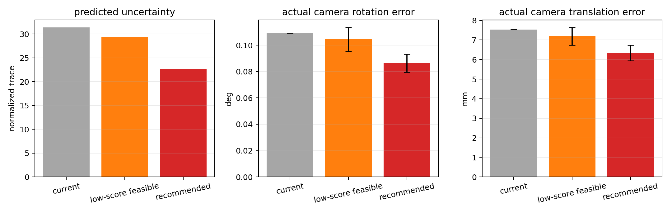
The reprojection RMSE stays near the pixel noise floor for both candidates, so it is not a sensitive placement metric. The camera-pose covariance and ground-truth pose error are more informative: the recommended board gives a larger predicted uncertainty reduction and a lower average camera-pose error after re-solving.
What This Demonstrates
The primitive observation is the camera-point edge $(c,p)$, while the optimized variables are camera and board poses. Centralized BA exploits this sparse structure and combines image observations with surveyed board priors to estimate both sets of poses. It is the default solver for an EOL station that can process all observations on one machine.
4.5 Vehicle Rig: Board Count and Placement Refinement
The previous synthetic scene places cameras around a workspace. A more EOL-like setup is a vehicle rig. In this experiment, the cameras are mounted on a car-like body with seven cameras: front wide, front narrow, left-front, right-front, left-rear, right-rear, and rear. The side cameras are crossed in position: the cameras named left-front and right-front are physically closer to the rear, while the cameras named left-rear and right-rear are physically closer to the front. This creates overlapping side views. Boards are sampled from uniform rectangular perimeter rings around the vehicle, then the number of selected boards is increased.
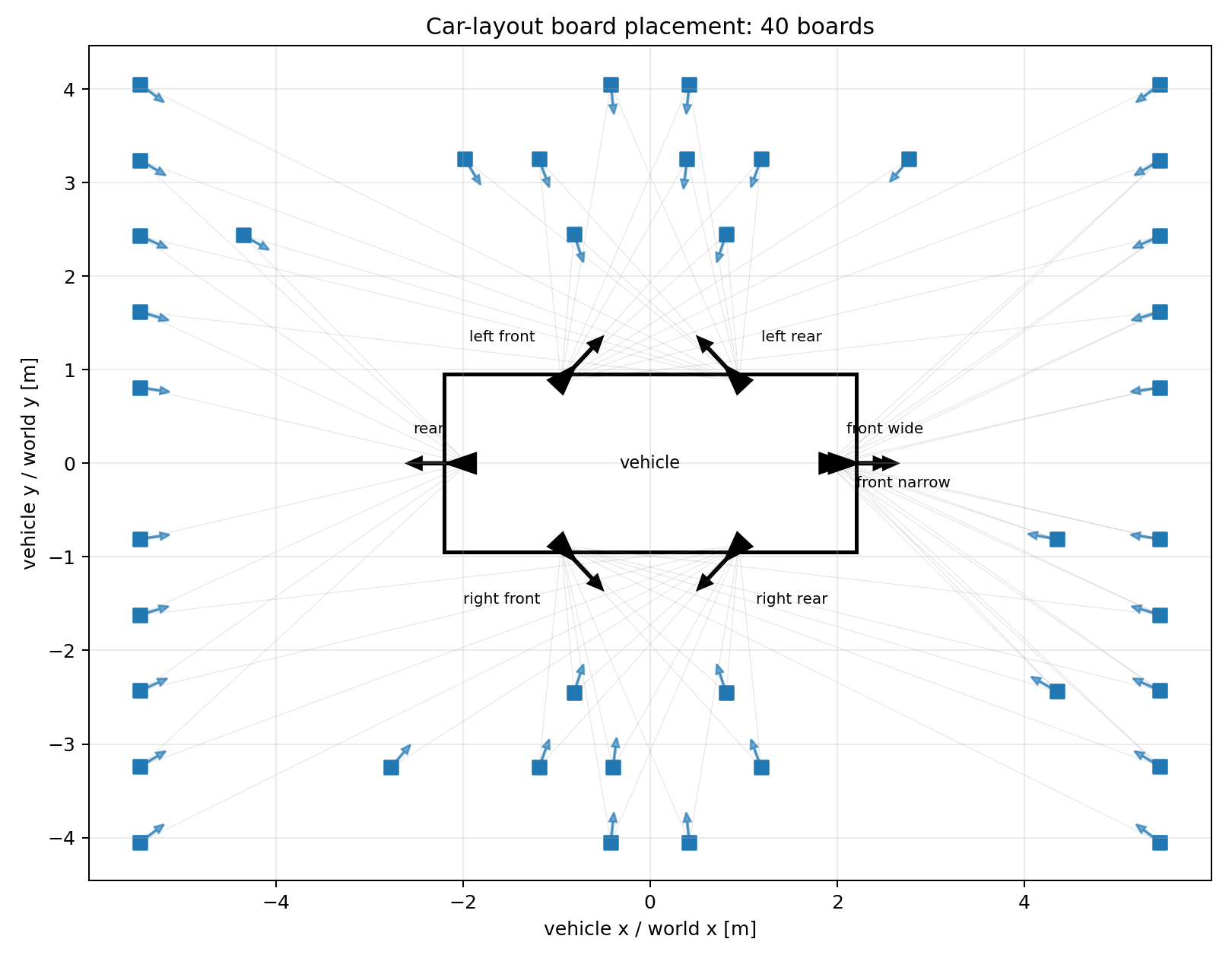
The visibility matrix for the 40-board case is intentionally sparse. Each board is visible to a subset of cameras, and each camera sees the boards in its sector. The side overlap is present: in this run, 7 boards are seen by both left-side cameras and 7 boards are seen by both right-side cameras.
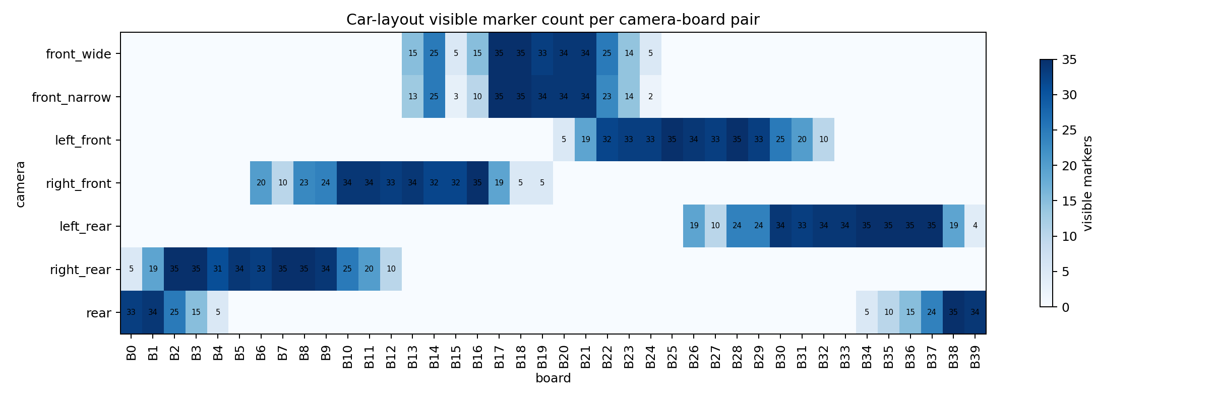
The centralized bundle-adjustment results for the board-count sweep are:
| Boards | Observations | Camera-Board Pairs | Central RMSE (px) | Central Runtime (s) |
|---|---|---|---|---|
| 8 | 481 | 18 | 1.0703 | 0.9360 |
| 12 | 656 | 28 | 1.0790 | 1.2224 |
| 16 | 893 | 34 | 1.0465 | 1.2350 |
| 24 | 1327 | 54 | 1.0338 | 2.5531 |
| 32 | 1765 | 72 | 1.0451 | 2.3942 |
| 40 | 2185 | 89 | 1.0391 | 1.6327 |
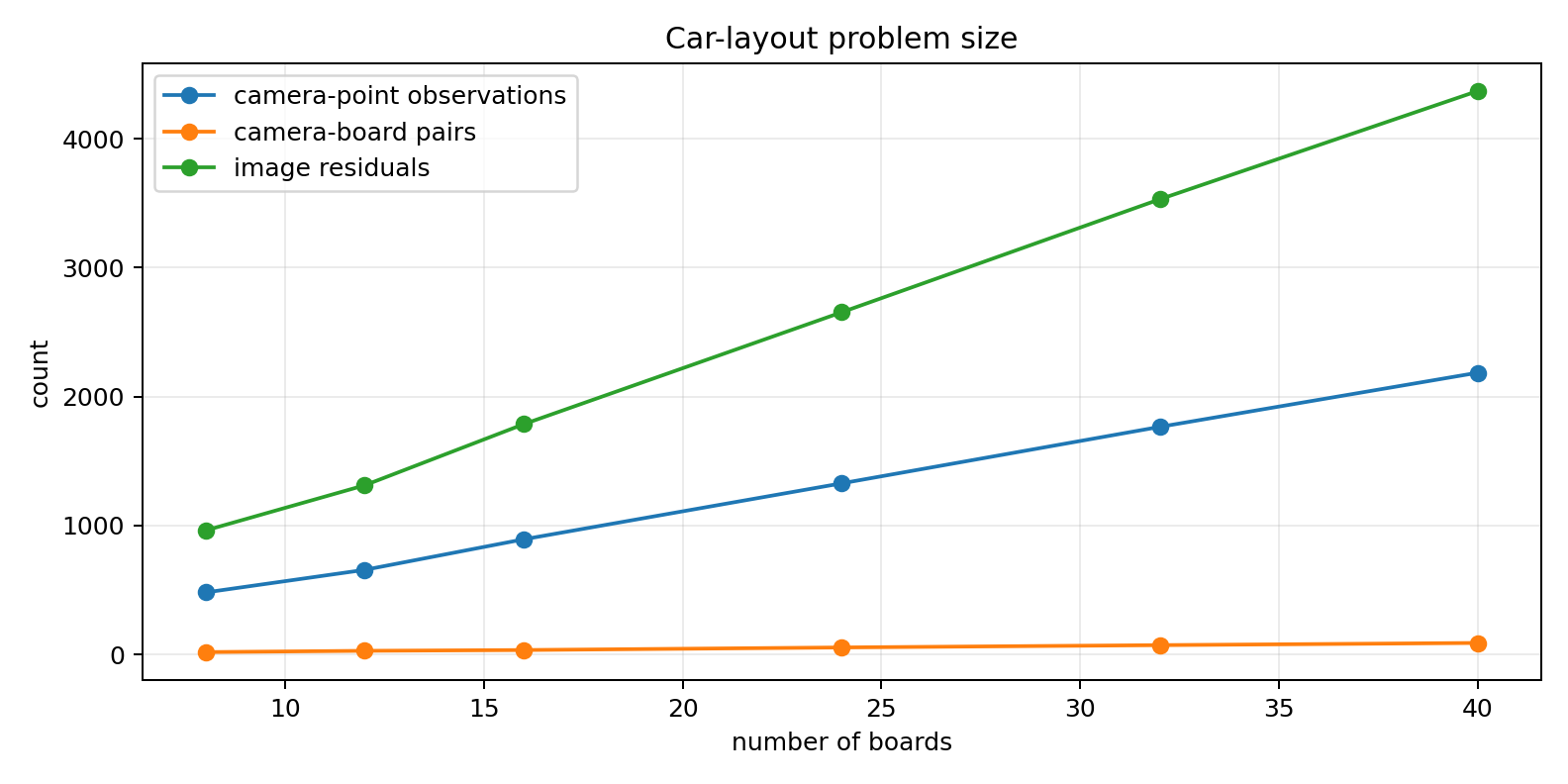
As the number of boards grows, camera error improves strongly at first. In this run, centralized BA goes from $0.1033^\circ$ and $7.0$ mm at 8 boards to $0.0412^\circ$ and $2.5$ mm at 32 boards. Additional boards mainly add redundancy, so the error plateaus near the pixel-noise and world-measurement limits.
This sweep also tells us how to use the placement-guidance method. The useful signal is not only the reprojection RMSE, because all layouts are near the pixel noise floor. The useful signal is that the 40-board uniform layout has more measurements than the 32-board layout, but worse camera-pose accuracy:
| Boards | Observations | Camera-Board Pairs | Central RMSE (px) | Central Camera Rot. (deg) | Central Camera Trans. (mm) |
|---|---|---|---|---|---|
| 24 | 1327 | 54 | 1.0338 | 0.0392 | 3.21 |
| 32 | 1765 | 72 | 1.0451 | 0.0412 | 2.49 |
| 40 | 2185 | 89 | 1.0391 | 0.0497 | 3.44 |
So the 40-board case is not limited by board count. It is limited by where those boards put information into the camera graph. The replacement experiment therefore keeps the board budget fixed at 40 and uses the solved 40-board state to ask a more targeted question: which candidate board poses would reduce the remaining camera-pose covariance the most?
The 40-board solution also identifies which camera directions are still weak. In the centralized BA result, the rear camera and the wide front camera remain larger-error poses than most side cameras:
| Camera | Rotation Error (deg) | Translation Error (mm) |
|---|---|---|
| front wide | 0.0703 | 4.63 |
| front narrow | 0.0197 | 1.81 |
| left front | 0.0120 | 1.03 |
| right front | 0.0238 | 3.64 |
| left rear | 0.0748 | 3.66 |
| right rear | 0.0272 | 2.15 |
| rear | 0.1205 | 7.18 |
This is why the guidance step does not simply spread boards more uniformly. It uses the solved uniform layout to score how each candidate board would couple the remaining uncertain cameras to the rest of the rig after board poses are marginalized.
Jacobian-Guided Refinement of the 40-Board Layout
The 40-board uniform layout can also be treated as the starting point for the board-placement guidance method. Here the goal is not to add one more board, but to replace the 40 boards with a better 40-board set using the solved uniform layout as the current calibration state.
The adjustment loop is:
- Solve the original uniform 40-board layout with centralized BA.
- Build the Schur-marginalized camera-pose information matrix from that solved state.
- Generate the same perimeter-ring candidate board poses used by the vehicle experiment.
- For each candidate, predict visible marker observations using the solved camera poses, build the candidate Jacobian, marginalize the candidate board pose, and score the candidate by camera covariance reduction.
- Start from the exact 40 initial board positions and evaluate one-for-one swaps: remove one existing board, add one candidate, and keep the swap only if the predicted camera covariance improves.
- Repeat the swap search until no candidate swap improves the Schur-marginalized camera-pose trace.
- Re-simulate noisy image and surveyed-world measurements for the refined board placement, then solve the calibration again.
For one candidate board pose $g$, the method linearizes the image residuals at the solved camera poses from the initial 40-board layout. Its camera-pose information contribution is computed after marginalizing the candidate board pose:
$$ \Lambda_g = J_c^\top W J_c - J_c^\top W J_b \left(J_b^\top W J_b\right)^{-1} J_b^\top W J_c . $$For a one-for-one replacement, the predicted score is the reduction in the normalized camera covariance trace after replacing an existing board contribution $\Lambda_r$ with $\Lambda_g$. This means the method is not just counting visible corners. It asks whether the new board’s Jacobian directions reduce the weak camera-pose modes left by the solved uniform layout.
As a concrete example, start from the blue-square 40-board top-down layout above. The initial board B5 corresponds to candidate G033 at $(-2.77,-3.25)$ m. It is visible from only one camera in the initial solution, and adding that pose alone would reduce the current camera covariance trace by only $0.25\%$. The highest-scoring unused candidate is G021 at $(-3.25,-0.82)$ m. It is visible from two cameras and, more importantly, its Jacobian couples a weak side/rear direction to the rest of the rig, giving a $23.7\%$ one-board trace reduction. The first greedy replacement therefore moves B5 to G021, while keeping the board normal pointed toward the vehicle. The predicted normalized trace drops from $4.1914$ to $3.2031$ after this one swap.
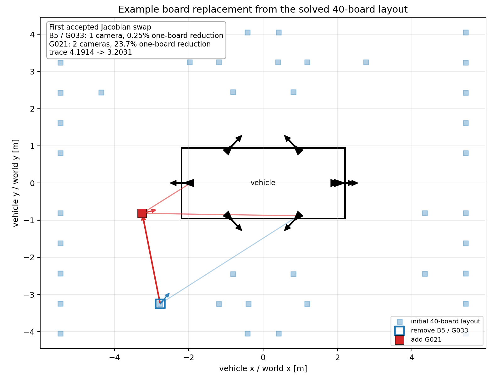
B5/G033 and add the Jacobian-scored candidate G021.The score map below is the direct analog of the earlier board-placement guidance plot. Color shows the single-board trace reduction if that candidate is added to the solved uniform layout. Red squares are the final 40-board refined placement after the swap search. Some red squares have modest single-board scores because the final set is produced by cumulative swaps, not by independently taking the top 40 one-board candidates.
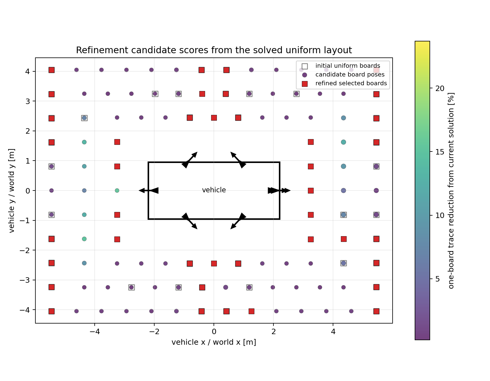
The highest single-board candidate scores are concentrated near side-overlap regions, where a board couples multiple cameras strongly:
| Candidate | x (m) | y (m) | Visible Cameras | Marker Observations | One-Board Trace Reduction | Refined Set | Initially Used |
|---|---|---|---|---|---|---|---|
| G021 | -3.25 | -0.82 | 2 | 30 | 23.7% | yes | no |
| G024 | 3.25 | 0.82 | 3 | 53 | 23.1% | yes | no |
| G025 | -3.25 | 0.82 | 2 | 30 | 22.8% | yes | no |
| G019 | -3.25 | -1.63 | 2 | 35 | 22.2% | yes | no |
| G020 | 3.25 | -0.82 | 3 | 55 | 21.5% | yes | no |
| G026 | 3.25 | 1.63 | 3 | 45 | 21.1% | yes | no |
| G027 | -3.25 | 1.63 | 2 | 35 | 21.0% | yes | no |
| G018 | 3.25 | -1.63 | 3 | 45 | 18.7% | yes | no |
The actual refinement performs 14 beneficial swaps and keeps 26 of the original 40 board positions:
| Step | Remove | Add | Added Position (x,y) m | Trace After | Reduction From Initial |
|---|---|---|---|---|---|
| 1 | B5 (G033) | G021 | (-3.25, -0.82) | 3.2031 | 23.6% |
| 2 | B25 (G046) | G024 | (3.25, 0.82) | 2.2513 | 46.3% |
| 3 | B33 (G034) | G020 | (3.25, -0.82) | 2.0222 | 51.8% |
| 4 | B39 (G105) | G025 | (-3.25, 0.82) | 1.8508 | 55.8% |
| 5 | B0 (G101) | G009 | (0.00, -2.45) | 1.7680 | 57.8% |
| 6 | B19 (G100) | G026 | (3.25, 1.63) | 1.6909 | 59.7% |
| 7 | B27 (G042) | G008 | (0.00, 2.45) | 1.6189 | 61.4% |
| 8 | B20 (G104) | G018 | (3.25, -1.63) | 1.5642 | 62.7% |
| 9 | B7 (G037) | G019 | (-3.25, -1.63) | 1.5138 | 63.9% |
| 10 | B35 (G065) | G027 | (-3.25, 1.63) | 1.4756 | 64.8% |
| 11 | B18 (G056) | G022 | (3.25, 0.00) | 1.4634 | 65.1% |
| 12 | B12 (G043) | G083 | (1.26, -4.05) | 1.4564 | 65.3% |
| 13 | B32 (G036) | G038 | (-0.40, 3.25) | 1.4510 | 65.4% |
| 14 | B16 (G052) | G054 | (4.35, -1.62) | 1.4493 | 65.4% |
The predicted information metric improves before any noisy re-simulation:
| Layout | Normalized Trace | Mean Rot. Std. (deg) | Mean Trans. Std. (mm) | Trace Reduction |
|---|---|---|---|---|
| initial uniform | 4.1914 | 0.0290 | 1.5888 | 0.0% |
| refined placement | 1.4493 | 0.0185 | 0.9261 | 65.4% |
The matrix view shows why the refinement helps: the refined placement increases the Schur-marginalized camera-pose information and strengthens several camera-camera coupling blocks after board poses are marginalized.
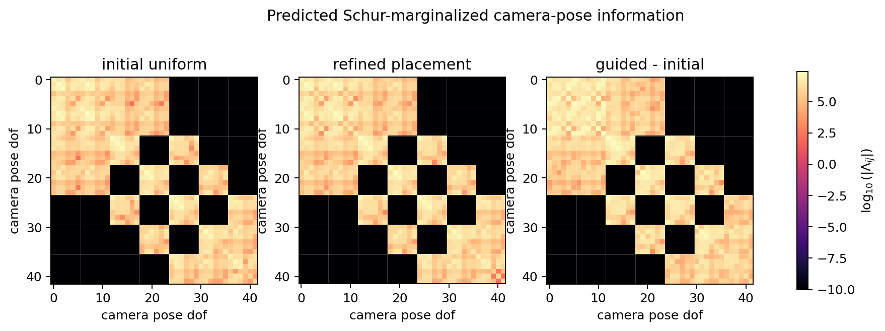
The per-camera uncertainty view shows that the improvement is not only global trace reduction. The front and rear cameras receive the largest predicted uncertainty reduction, while the side cameras also improve.
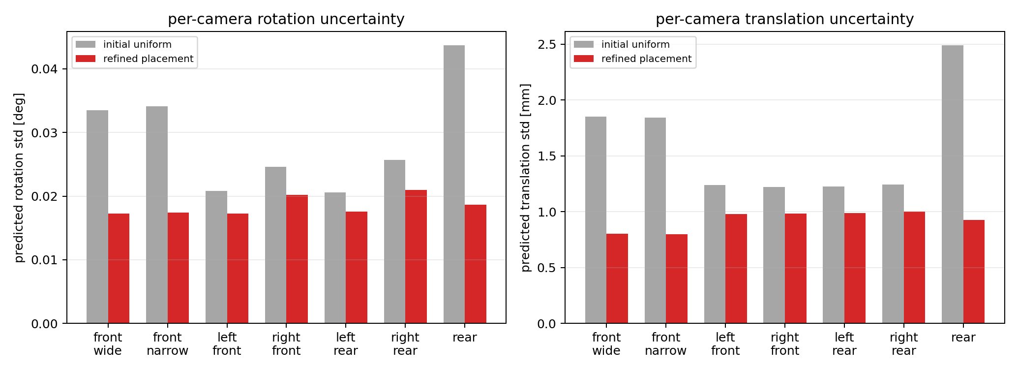
The new board positions are shown below. Gray hollow squares are the original uniform 40-board positions; red squares are the refined positions, with arrows showing board normals.
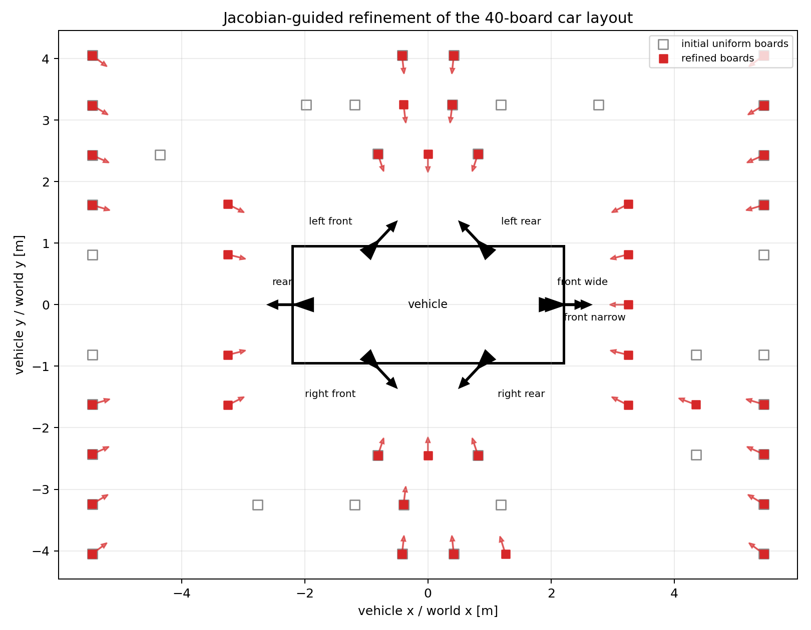
After re-simulating noisy image and surveyed-world measurements with the refined board set, centralized BA reduces mean camera rotation error by 58.9% and translation error by 47.5%. Reprojection RMSE stays near the pixel noise floor, so camera-pose error is the more informative metric here.
| Method | Initial RMSE (px) | Refined RMSE (px) | Initial Camera Rot. (deg) | Refined Camera Rot. (deg) | Rot. Reduction | Initial Camera Trans. (mm) | Refined Camera Trans. (mm) | Trans. Reduction |
|---|---|---|---|---|---|---|---|---|
| Centralized BA | 1.0391 | 1.0391 | 0.0497 | 0.0205 | 58.9% | 3.44 | 1.81 | 47.5% |
The exact refined board centers and horizontal normal directions are:
| Board | x (m) | y (m) | z (m) | Normal x | Normal y | Visible Cameras | Marker Observations | Original Board |
|---|---|---|---|---|---|---|---|---|
| B0 | -5.45 | -1.62 | 1.16 | 0.958 | 0.285 | 2 | 55 | yes |
| B1 | -5.45 | -2.43 | 1.08 | 0.913 | 0.407 | 2 | 60 | yes |
| B2 | -5.45 | -3.24 | 1.12 | 0.860 | 0.511 | 2 | 50 | yes |
| B3 | -5.45 | -4.05 | 1.08 | 0.803 | 0.596 | 2 | 40 | yes |
| B4 | -0.81 | -2.45 | 1.12 | 0.315 | 0.949 | 2 | 55 | yes |
| B5 | -0.40 | -3.25 | 1.08 | 0.121 | 0.992 | 2 | 60 | yes |
| B6 | -0.42 | -4.05 | 1.08 | 0.103 | 0.994 | 2 | 60 | yes |
| B7 | 0.42 | -4.05 | 1.16 | -0.103 | 0.994 | 2 | 60 | yes |
| B8 | 0.81 | -2.45 | 1.16 | -0.315 | 0.949 | 2 | 55 | yes |
| B9 | 5.45 | -3.24 | 1.08 | -0.860 | 0.511 | 3 | 65 | yes |
| B10 | 5.45 | -2.43 | 1.16 | -0.913 | 0.407 | 3 | 85 | yes |
| B11 | 5.45 | -4.05 | 1.16 | -0.803 | 0.596 | 3 | 43 | yes |
| B12 | 5.45 | -1.62 | 1.12 | -0.958 | 0.285 | 3 | 90 | yes |
| B13 | 5.45 | 1.62 | 1.08 | -0.958 | -0.285 | 3 | 90 | yes |
| B14 | 5.45 | 2.43 | 1.16 | -0.913 | -0.407 | 3 | 85 | yes |
| B15 | 5.45 | 3.24 | 1.12 | -0.860 | -0.511 | 3 | 65 | yes |
| B16 | 5.45 | 4.05 | 1.12 | -0.803 | -0.596 | 3 | 43 | yes |
| B17 | 0.81 | 2.45 | 1.12 | -0.315 | -0.949 | 2 | 55 | yes |
| B18 | 0.40 | 3.25 | 1.12 | -0.121 | -0.992 | 2 | 60 | yes |
| B19 | 0.42 | 4.05 | 1.12 | -0.103 | -0.994 | 2 | 60 | yes |
| B20 | -0.42 | 4.05 | 1.16 | 0.103 | -0.994 | 2 | 60 | yes |
| B21 | -0.81 | 2.45 | 1.08 | 0.315 | -0.949 | 2 | 55 | yes |
| B22 | -5.45 | 4.05 | 1.16 | 0.803 | -0.596 | 2 | 40 | yes |
| B23 | -5.45 | 3.24 | 1.16 | 0.860 | -0.511 | 2 | 50 | yes |
| B24 | -5.45 | 2.43 | 1.08 | 0.913 | -0.407 | 2 | 60 | yes |
| B25 | -5.45 | 1.62 | 1.12 | 0.958 | -0.285 | 2 | 55 | yes |
| B26 | -3.25 | -0.82 | 1.08 | 0.970 | 0.244 | 2 | 30 | no |
| B27 | 3.25 | 0.82 | 1.08 | -0.970 | -0.244 | 3 | 53 | no |
| B28 | 3.25 | -0.82 | 1.16 | -0.970 | 0.244 | 3 | 55 | no |
| B29 | -3.25 | 0.82 | 1.12 | 0.970 | -0.244 | 2 | 30 | no |
| B30 | 0.00 | -2.45 | 1.08 | -0.000 | 0.999 | 2 | 70 | no |
| B31 | 3.25 | 1.63 | 1.16 | -0.893 | -0.449 | 3 | 45 | no |
| B32 | 0.00 | 2.45 | 1.16 | -0.000 | -0.999 | 2 | 70 | no |
| B33 | 3.25 | -1.63 | 1.08 | -0.893 | 0.449 | 3 | 45 | no |
| B34 | -3.25 | -1.63 | 1.12 | 0.893 | 0.449 | 2 | 35 | no |
| B35 | -3.25 | 1.63 | 1.08 | 0.893 | -0.449 | 2 | 35 | no |
| B36 | 3.25 | 0.00 | 1.12 | -1.000 | -0.000 | 2 | 63 | no |
| B37 | 1.26 | -4.05 | 1.12 | -0.297 | 0.955 | 2 | 45 | no |
| B38 | -0.40 | 3.25 | 1.16 | 0.121 | -0.992 | 2 | 60 | no |
| B39 | 4.35 | -1.62 | 1.08 | -0.937 | 0.350 | 3 | 70 | no |
4.6 What the Experiments Establish
The one-board experiment demonstrates continuous physical pose optimization and exposes the translation-rotation trade-off behind an off-centre result. The two-camera experiments add shared geometry and uncertain board poses. The workspace and vehicle experiments then test sparse calibration, partial visibility, board count, and fixed-budget placement refinement.
Across these cases, the calibration loss estimates poses, while the marginalized information predicts which physical observations will improve those estimates. Reprojection RMSE alone is not a reliable placement objective. The numerical optima remain conditional on the assumed world anchor, camera model, corner noise, and feasible workspace.
Appendix A. Geometric Preprocessing and Board Survey Refinement
These derivations support initialization and the fixed-board image-processing experiment in Section 4.2. Ray-plane reconstruction is an optional geometric route, not a required residual in the reprojection-based solver of Section 2.
A.1 Optional Geometric Pipeline
Do single camera intrinsic calibration
Measure each corner in the world coordinate
Refine the corners’ coordinates according to board constraints (plane, parallel, equally spaced)
Find the plane equation in the world coordinate
Initialize each camera’s extrinsic parameters by solving the perspective-n-point (PnP) problem
Estimate the 3D coordinates by the intersection of the image ray and board plane
Construct the objective loss function from pixel reprojection residuals that share board-generated marker points, plus optional world-point or pose priors
A.2 Refine Surveyed Corners Using Board Constraints
Assume the center of the board is located at the origin of a local coordinate, $(0,0,0)^\top$, the corner coordinate is located at $\{\mathbf{x}_i\}^N_{i=1}$, then the board normal is $(0,0,1)^\top$. Assume the board is transformed to the world coordinate by rotation, $\mathbf{R}$, and translation, $\mathbf{t}$. We have the observed coordinates $\{\hat{\mathbf{y}}_i\}$. Then we minimize the objective:
$$ (\mathbf{R}^*, \mathbf{t}^*) = \underset{\mathbf{R}\in SO(3),\,\mathbf{t}\in\mathbb R^3}{\arg\min} \sum_i \left\| \hat{\mathbf{y}}_i-(\mathbf{R}\mathbf{x}_i+\mathbf{t}) \right\|^2, \qquad \mathbf{y}_i^*=\mathbf{R}^*\mathbf{x}_i+\mathbf{t}^*. $$Because the board-corner correspondences are already known, this is an orthogonal Procrustes/Kabsch rigid-alignment problem. ICP is needed only when the correspondences also have to be estimated.
If the board-frame origin is at the board center, then the center of the board is $\mathbf{x}_0=\mathbf{t}^*$, and the normal of the board is $\mathbf{R}^*[0, 0, 1]^\top$.
Now we have refined board corners in the world coordinates, i.e., $\{\mathbf{y}_i^*\}^N_{i=1}$.
Unknown Board Dimension
If we do not have the board dimension, then we can directly fit the plane using the measured corners, $\{\mathbf{x}_i\}^N_{i=1}$ (with a slight abuse of notation). Use the plane convention $\mathbf{n}^\top \mathbf{x} + c = 0$ (with unit normal vector, i.e., $\|\mathbf{n}\| = 1$). Then we can solve for $\mathbf{n}$ and $c$ by minimizing the following objective:
$$ \underset{\mathbf{n}, c}{\text{argmin}} \frac{1}{N}\sum_i \|\mathbf{n}^\top \mathbf{x}_i + c\|^2 \\ \text{s.t. } \|\mathbf{n}\| = 1 $$For any fixed $\mathbf{n}$, taking derivative with respect to $c$ and setting it to zero, we have:
$$ c = -\frac{1}{N} \sum_i \mathbf{n}^\top \mathbf{x}_i = - \mathbf{n}^\top \bar{\mathbf{x}} $$where $\bar{\mathbf{x}} = \frac{1}{N} \sum_i \mathbf{x}_i$ is the mean of the measured corners.
So, the objective function becomes:
$$ \begin{aligned} &\frac{1}{N}\sum_i \|\mathbf{n}^\top (\mathbf{x}_i - \bar{\mathbf{x}})\|^2 \\ &= \frac{1}{N}\mathbf{n}^\top \left(\sum_i (\mathbf{x}_i - \bar{\mathbf{x}})(\mathbf{x}_i - \bar{\mathbf{x}})^\top\right) \mathbf{n} \\ & = \mathbf{n}^\top \mathbf{\Sigma}_x \mathbf{n} \end{aligned} $$where $\mathbf{\Sigma}_x = \frac{1}{N} \sum_i (\mathbf{x}_i - \bar{\mathbf{x}})(\mathbf{x}_i - \bar{\mathbf{x}})^\top$ is the biased sample covariance matrix of the measured corners.
Considering $\|\mathbf{n}\| = 1$, $\mathbf{n}$ is the eigenvector of $\mathbf{\Sigma}_x$ corresponding to its smallest eigenvalue.
The refined corners’ coordinates are the projection of the measured corners on the plane, which can be written as:
$$ \mathbf{y}_i = \mathbf{x}_i - \mathbf{n}^\top (\mathbf{x}_i - \bar{\mathbf{x}}) \mathbf{n} = \mathbf{x}_i - (\mathbf{n}^\top\mathbf{x}_i + c)\mathbf{n}. $$which has clear geometric meaning: the measured corners minus the signed distance along the plane normal. The sign of $\mathbf n$ remains arbitrary as long as $c$ is changed consistently.
Appendix B. Ray-Plane Geometry and Optional Residuals
The first two derivations use world-to-camera extrinsics $(R,t)$: $X^C=RX^W+t$. Relative to the main article’s camera-to-world pose, $R=(R^C)^\top$ and $t=-(R^C)^\top t^C$. The coordinate conversion is explicit here so that the main formulation retains one consistent local-to-world convention.
B.1 Closed-Form Ray-Plane Intersection
We are given a 3D plane:
$$\mathbf{n}^\top \mathbf{x} + c = 0,$$and a camera model with the projection equation:
$$d\, \mathbf{u} = \mathbf{K} (\mathbf{R}\, \mathbf{x} + \mathbf{t}),$$where:
- $\mathbf{u} \in \mathbb{R}^3$ is the homogeneous image coordinate (usually $\mathbf{u} = [u, v, 1]^\top$)
- $d$ is an unknown scale (depth) factor
- $\mathbf{K}$ is the camera intrinsic matrix
- $\mathbf{R}$ and $\mathbf{t}$ are the rotation and translation (extrinsic parameters) of the camera
- $\mathbf{x} \in \mathbb{R}^3$ is the 3D point we wish to recover
Our goal is to find $\mathbf{x}$ in terms of the known quantities $\mathbf{u}, \mathbf{K}, \mathbf{R}, \mathbf{t}, \mathbf{n},$ and $c$.
Rewrite the Projection Equation
$$\mathbf{x} = \mathbf{R}^\top \left(d\,\mathbf{K}^{-1} \mathbf{u} - \mathbf{t}\right).$$However, the scale factor $d$ is still unknown.
Use the Plane Constraint to Solve for $d$
Since $\mathbf{x}$ lies on the plane, it must satisfy:
$$\mathbf{n}^\top \mathbf{x} + c = 0.$$Substitute the expression we just found for $\mathbf{x}$:
$$\mathbf{n}^\top \Bigl(\mathbf{R}^\top (d\,\mathbf{K}^{-1} \mathbf{u} - \mathbf{t})\Bigr) + c = 0.$$Expanding the scalar equation gives
$$ d\,\mathbf{n}^\top\mathbf{R}^\top\mathbf{K}^{-1}\mathbf{u}- \mathbf{n}^\top\mathbf{R}^\top\mathbf{t} + c = 0. $$Now solve for $d$:
$$d = \frac{\mathbf{n}^\top \mathbf{R}^\top \mathbf{t} - c}{\mathbf{n}^\top \mathbf{R}^\top \mathbf{K}^{-1} \mathbf{u}}.$$Note: It is important that $\mathbf{n}^\top \mathbf{R}^\top \mathbf{K}^{-1} \mathbf{u} \neq 0$ so that the division is valid (this means that the back-projected ray is not parallel to the plane).
Substitute the expression for $d$ back into the equation for $\mathbf{x}$:
$$\mathbf{x} = \mathbf{R}^\top \left( \frac{\mathbf{n}^\top \mathbf{R}^\top \mathbf{t} - c}{\mathbf{n}^\top \mathbf{R}^\top \mathbf{K}^{-1} \mathbf{u}}\, \mathbf{K}^{-1} \mathbf{u} - \mathbf{t} \right).$$B.2 Ray-Plane Intersection as an Optimization Problem
If we write the ray-plane intersection as an optimization, the pixel-space objective should be dimensionally consistent:
$$ \min_{\mathbf{x}} \left\| \mathbf{u}- \pi\left( \mathbf{K}(\mathbf{R}\mathbf{x}+\mathbf{t}) \right) \right\|^2 \tag{1} $$subject to the plane constraint
$$ \mathbf{n}^\top \mathbf{x} + c = 0, $$where $\mathbf{u}\in\mathbb R^2$ is a pixel coordinate and
$$ \pi([a,b,d]^\top)= \begin{bmatrix} a/d\\ b/d \end{bmatrix}. $$If $\mathbf{u}$ instead denotes normalized undistorted image coordinates, then $\mathbf{K}$ can be omitted and the ray direction is $\mathbf{R}^{-1}[\mathbf{u}^\top,1]^\top$.
Even when the measured image coordinate $\mathbf{u}$ is noisy, the pinhole camera model combined with the infinite plane constraint induces a homography from the plane to the image. For any image coordinate, there is a back-projected ray, and if that ray intersects the plane, the corresponding 3D point projects exactly back to the same coordinate. Therefore, Eq. (1) has minimum value zero whenever the ray intersects the plane. By itself, ray-plane intersection does not correct noisy image measurements; board-marker geometry or other multi-view observations must provide the denoising constraint.
- Parameterizing the Back‐Projection Ray
For normalized image coordinates, any 3D point $\mathbf{x}$ whose projection is $\mathbf{u}$ must satisfy
$$ \mathbf{R}\mathbf{x}+\mathbf{t}= \lambda \begin{pmatrix} \mathbf{u}\\ 1 \end{pmatrix}. $$Solving for $\mathbf{x}$ gives
$$ \mathbf{x} = \mathbf{R}^{-1} \Bigl( \lambda \begin{pmatrix} \mathbf{u} \\ 1 \end{pmatrix} - \mathbf{t} \Bigr). $$It is convenient to define the camera center in world coordinates as
$$ \mathbf{x}_c = -\mathbf{R}^{-1}\mathbf{t}, $$and to introduce the direction vector
$$ \mathbf{d} = \mathbf{R}^{-1}\begin{pmatrix} \mathbf{u} \\ 1 \end{pmatrix}. $$Thus, the 3D point $\mathbf{x}$ can be written as
$$ \mathbf{x} = \mathbf{x}_c + \lambda \mathbf{d}. $$All points of this form project exactly to $\mathbf{u}$, which means the optimal value of Eq. (1) is zero
- Enforcing the Plane Constraint
Since $\mathbf{x}$ must lie on the plane, we impose
$$ \mathbf{n}^\top \mathbf{x} + c = 0. $$Substitute $\mathbf{x} = \mathbf{x}_c + \lambda\mathbf{d}$ into the plane equation:
$$ \mathbf{n}^\top \Bigl( \mathbf{x}_c + \lambda\mathbf{d} \Bigr) + c = 0. $$Expanding, we obtain
$$ \mathbf{n}^\top \mathbf{x}_c + \lambda \mathbf{n}^\top \mathbf{d} + c = 0. $$Recalling that $\mathbf{x}_c = -\mathbf{R}^{-1}\mathbf{t}$, the equation becomes
$$ - \mathbf{n}^\top \mathbf{R}^{-1}\mathbf{t} + \lambda \mathbf{n}^\top \mathbf{d} + c = 0. $$Solving for $\lambda$, we have
$$ \lambda \mathbf{n}^\top \mathbf{d} = \mathbf{n}^\top \mathbf{R}^{-1}\mathbf{t} - c, $$or equivalently,
$$ \lambda = \frac{\mathbf{n}^\top \mathbf{R}^{-1}\mathbf{t} - c}{\mathbf{n}^\top \mathbf{d}} = \frac{\mathbf{n}^\top \mathbf{R}^{-1}\mathbf{t} - c}{\mathbf{n}^\top \mathbf{R}^{-1}\begin{pmatrix} \mathbf{u} \\ 1 \end{pmatrix}}, $$provided that $\mathbf{n}^\top \mathbf{d} \neq 0$.
A physically visible intersection also requires positive camera depth.
- The Final Solution
Substitute the value of $\lambda$ back into the expression for $\mathbf{x}$:
$$ \mathbf{x} = -\mathbf{R}^{-1}\mathbf{t} + \frac{\mathbf{n}^\top \mathbf{R}^{-1}\mathbf{t} - c}{\mathbf{n}^\top \mathbf{R}^{-1}\begin{pmatrix} \mathbf{u} \\ 1 \end{pmatrix}} \mathbf{R}^{-1}\begin{pmatrix} \mathbf{u} \\ 1 \end{pmatrix}. $$This is the unique 3D point on the plane $\mathbf{n}^\top \mathbf{x} + c = 0$ selected by the measured ray, provided the ray is not parallel to the plane and the depth is positive.
- Summary
a. Back‐Projection: The projection model
$$ \mathbf{x} \mapsto \frac{\mathbf{R}\mathbf{x} + \mathbf{t}}{\mathbf{e}^\top (\mathbf{R}\mathbf{x} + \mathbf{t})} $$is a homography when restricted to the plane. Hence, every point along the ray
$$ \mathcal{R}(\mathbf{u}) = \Bigl\{ \mathbf{x} = -\mathbf{R}^{-1}\mathbf{t} + \lambda \mathbf{R}^{-1}\begin{pmatrix} \mathbf{u} \\ 1 \end{pmatrix} : \lambda \in \mathbb{R} \Bigr\} $$projects to $\mathbf{u}$.
b. Plane Intersection: The plane constraint $\mathbf{n}^\top \mathbf{x} + c = 0$ uniquely determines the scalar $\lambda$, and hence the unique point $\mathbf{x}$.
Thus, the final answer is
$$ \boxed{ \mathbf{x} = -\mathbf{R}^{-1}\mathbf{t} + \frac{\mathbf{n}^\top \mathbf{R}^{-1}\mathbf{t} - c}{\mathbf{n}^\top \mathbf{R}^{-1}\begin{pmatrix} \mathbf{u} \\ 1 \end{pmatrix}} \mathbf{R}^{-1}\begin{pmatrix} \mathbf{u} \\ 1 \end{pmatrix}. } $$B.3 Optional Board-Plane Residual
The main formulation uses reprojection error. As an optional alternative, inverse ray-plane intersection gives the point where a back-projected image ray intersects a known plane, provided the ray is not parallel to the plane. This subsection returns to the local-to-world camera pose convention used in the main article.
For board $b$, its world-frame plane is
$$ n_b^\top X+c_b=0, $$where
$$ n_b=R^B_b e_3, \qquad c_b=-n_b^\top t^B_b, \qquad e_3= \begin{bmatrix} 0\\0\\1 \end{bmatrix}. $$Camera $c$’s center in world coordinates is now directly:
$$ \boxed{ o_c=t^C_c. } $$For homogeneous image coordinate
$$ \tilde u_{cp}= \begin{bmatrix} u_{cp}\\ v_{cp}\\ 1 \end{bmatrix}, $$the ray direction in camera coordinates is
$$ d_{cp}^{C} = K_c^{-1}\tilde u_{cp}. $$The same direction in world coordinates is
$$ \boxed{ d_{cp}^{W} = R^C_c d_{cp}^{C}. } $$The ray-plane intersection is
$$ \boxed{ \phi_{cp}(T^C_c,T^B_b) = o_c - \frac{n_b^\top o_c+c_b} {n_b^\top d_{cp}^{W}} d_{cp}^{W}. } $$The board-generated world point is
$$ \boxed{ X_p^W=R^B_b q_p+t^B_b. } $$The post-style residual would be
$$ \boxed{ r_{cp}^{\text{ray}} = P_b^\top \left[ \phi_{cp}(T^C_c,T^B_{\beta(p)}) - \left( R^B_{\beta(p)} q_p+t^B_{\beta(p)} \right) \right], } $$where
$$ P_b= \begin{bmatrix} R^B_b e_1 & R^B_b e_2 \end{bmatrix} \in\mathbb R^{3\times2} $$is the tangent basis of the board plane.
I recommend using the tangent-plane residual, not the full 3D residual, because both points are supposed to lie on the board plane and the meaningful error is along the board surface.
However, the reprojection objective is usually preferable because pixel noise is naturally modeled in image coordinates. The ray-plane residual requires converting pixel uncertainty into board-plane uncertainty, which depends on viewing angle and can become ill-conditioned when
$$ n_b^\top d_{cp}^{W}\approx 0. $$Appendix C. Alternative Design Formulations
The main article uses camera-uncertainty minimization. This appendix retains alternative criteria and derivations for readers who need a different design objective or a discrete placement budget.
C.1 Single-Board Objective and Tolerance Scaling
A direct next-board-placement problem is
$$ \boxed{ (T^B_b)^* = \underset{T^B_b\in\mathcal F}{\arg\min} \; \operatorname{tr} \left( D\Sigma_C(T^B_b)D^\top \right), } $$where $\mathcal F$ is the feasible set of board poses, and $D$ normalizes translation and rotation by required tolerances. For a single camera pose, one example is
$$ D = \operatorname{diag} \left( 1/\tau_x,\, 1/\tau_y,\, 1/\tau_z,\, 1/\tau_{\mathrm{roll}},\, 1/\tau_{\mathrm{pitch}},\, 1/\tau_{\mathrm{yaw}} \right). $$For multiple cameras, use the corresponding block-diagonal normalization.
Other useful criteria are the D-optimal score
$$ \boxed{ \max_{T^B_b\in\mathcal F} \log\det\Lambda_C(T^B_b), } $$which reduces the overall uncertainty volume, and the E-optimal score
$$ \boxed{ \max_{T^B_b\in\mathcal F} \lambda_{\min} \left( D^{-T}\Lambda_C(T^B_b)D^{-1} \right), } $$which improves the least observable camera-pose direction. For extrinsic calibration, the E-optimal criterion is often the more practical one, because a calibration can have a small average error while still containing one poorly constrained combination, such as camera height and pitch.
C.2 Overview of Alternative Criteria
Other experimental-design objectives can be substituted:
$$ \text{D-optimal:}\qquad \underset{s\in\mathcal S}{\arg\max}\; \log\det \Lambda_\theta(s) - \lambda_{\mathrm{cost}}C_{\mathrm{place}}(s), $$$$ \text{E-optimal:}\qquad \underset{s\in\mathcal S}{\arg\max}\; \lambda_{\min} \left( D^{-T}\Lambda_\theta(s)D^{-1} \right) - \lambda_{\mathrm{cost}}C_{\mathrm{place}}(s), $$or a worst-camera objective:
$$ \underset{s\in\mathcal S}{\arg\min}\; \max_{c\in\mathcal C} \operatorname{tr} \left( D_c \Sigma_{\theta_c}(s)D_c^\top \right) + \lambda_{\mathrm{cost}}C_{\mathrm{place}}(s). $$C.3 Detailed Alternative Upper-Level Criteria
The A-optimal objective in (BL-A) minimizes the normalized trace of the predicted camera covariance. Other criteria are useful in different production settings.
D-optimal placement minimizes the uncertainty volume:
$$ \boxed{ s^\star = \underset{s\in\mathcal S}{\arg\max} \; \log\det \Lambda_\theta(s) - \lambda_{\mathrm{cost}}C_{\mathrm{place}}(s). } \tag{BL-D} $$Equivalently,
$$ s^\star = \underset{s\in\mathcal S}{\arg\min} \; - \log\det \Lambda_\theta(s) + \lambda_{\mathrm{cost}}C_{\mathrm{place}}(s). $$E-optimal placement improves the weakest observable camera-pose direction:
$$ \boxed{ s^\star = \underset{s\in\mathcal S}{\arg\max} \; \lambda_{\min} \left( D^{-T} \Lambda_\theta(s) D^{-1} \right) - \lambda_{\mathrm{cost}}C_{\mathrm{place}}(s). } \tag{BL-E} $$This is often useful for camera extrinsic calibration because the failure mode is usually not the average error, but one poorly constrained direction, such as height-pitch coupling or lateral-yaw coupling.
If every camera must satisfy a production tolerance, use a worst-camera objective:
$$ \boxed{ s^\star = \underset{s\in\mathcal S}{\arg\min} \; \max_{c\in\mathcal C} \operatorname{tr} \left( D_c \Sigma_{\theta_c}(s) D_c^\top \right) + \lambda_{\mathrm{cost}}C_{\mathrm{place}}(s). } \tag{BL-worst} $$This avoids a placement that helps some cameras but leaves one camera poorly calibrated.
C.4 Abstract Bilevel Form and Objective Choices
Putting the lower and upper levels together gives the clean abstract formulation:
$$ \boxed{ \begin{aligned} s^\star = \underset{s\in\mathcal S}{\arg\min} &\quad \mathcal U(x^\star(s),s) \\ \text{s.t.} &\quad x^\star(s) \in \underset{x}{\arg\min} \; \mathcal L(x;s), \end{aligned} } \tag{BL} $$where
$$ x= \left( \{T_c^C\}_{c=1}^C, \{T_b^B\}_{b=1}^B \right), $$and $\mathcal L(x;s)$ is the joint calibration objective. The upper objective can be chosen according to the available information.
If the goal is truly optimized residual, use
$$ \boxed{ \mathcal U_{\mathrm{res}}(x^\star,s) = \mathbb E \left[ \frac{1}{|\mathcal E(s)|} \mathcal L(x^\star(s);s) \right]. } $$If the study is a simulation and the ground-truth camera poses are known, use the actual camera-pose error:
$$ \boxed{ \mathcal U_{\mathrm{pose}}(x^\star,s) = \mathbb E \left[ \sum_c \left\| \operatorname{Log} \left( (T_c^{C,\mathrm{true}})^{-1} (T_c^C)^\star(s) \right) \right\|_{D_c^\top D_c}^2 \right]. } $$For a real calibration station, the most practical design objective is information-based:
$$ \boxed{ \mathcal U_{\mathrm{info}}(s) = \operatorname{tr} \left( D\Lambda_\theta(s)^{-1}D^\top \right). } $$For EOL board-placement design, $\mathcal U_{\mathrm{info}}(s)$ is preferable to optimized residual because it directly measures predicted camera-pose uncertainty.
C.5 Why Optimized Residual Is Not the Placement Objective
If the upper level literally minimizes the final optimized residual, the bilevel problem is
$$ \boxed{ \begin{aligned} s^\star = \underset{s\in\mathcal S}{\arg\min} &\quad \mathbb E_{\epsilon} \left[ \mathcal L(x^\star(s,\epsilon);s,\epsilon) \right] + \lambda_{\mathrm{cost}}\,C_{\mathrm{place}}(s) \\ \text{s.t.} &\quad x^\star(s,\epsilon) \in \underset{x}{\arg\min} \; \mathcal L(x;s,\epsilon). \end{aligned} } \tag{BL-residual} $$The normalized version is usually better:
$$ \boxed{ s^\star = \underset{s\in\mathcal S}{\arg\min} \; \mathbb E_{\epsilon} \left[ \frac{1}{|\mathcal E(s)|} \mathcal L(x^\star(s,\epsilon);s,\epsilon) \right] + \lambda_{\mathrm{cost}}\,C_{\mathrm{place}}(s). } \tag{BL-residual-normalized} $$The normalization prevents a placement with fewer visible markers from appearing artificially better only because it has fewer residual terms. However, residual minimization is not the best placement-design objective. In the noise-free case, many feasible board placements can achieve nearly zero residual. A low optimized reprojection error does not necessarily mean that the camera pose is accurately estimated. A degenerate placement can fit its own observations while leaving some camera-pose directions weakly observable.
This is why the more useful second-level problem is an optimal experimental design problem: choose board placements that minimize predicted camera-pose uncertainty.
C.6 Residual Value Function and Envelope Derivative
The residual-minimization bilevel problem can also be written with the value function
$$ V(s) = \min_x \mathcal L(x;s). $$Then
$$ \boxed{ s^\star = \underset{s\in\mathcal S}{\arg\min} \; V(s). } \tag{VF} $$If the lower-level solution is unique and smooth, the envelope theorem gives
$$ \boxed{ \nabla_s V(s) = \frac{\partial \mathcal L}{\partial s} \left( x^\star(s);s \right). } $$This is computationally convenient because the derivative of $x^\star(s)$ is not needed when the upper objective is exactly the optimized lower-level loss. For calibration placement design, however, $V(s)$ is usually not the best objective because minimized residual can be small even when the pose estimate is uncertain.
C.7 Fixed-Budget Discrete Board Selection
The 40-board replacement experiment in Section 4.5 is a discrete, fixed-budget approximation of the board-placement design problem. Let $\mathcal G$ be the finite set of candidate perimeter-board poses, let $\mathcal A\subset\mathcal G$ be the selected board set, and let $|\mathcal A|=40$. For each candidate $g$, compute its marginalized camera-pose information contribution
$$ \Delta\Lambda_g = J_{c,g}^\top W_g J_{c,g} - J_{c,g}^\top W_g J_{b,g} \left( J_{b,g}^\top W_g J_{b,g} \right)^{-1} J_{b,g}^\top W_g J_{c,g}. $$Then the fixed-budget subset problem is
$$ \mathcal A^\star = \underset{\mathcal A\subset\mathcal G,\;|\mathcal A|=40}{\arg\min} \; \operatorname{tr} \left[ D \left( \Lambda_0 + \sum_{g\in\mathcal A} \Delta\Lambda_g \right)^{-1} D^\top \right] + \lambda_{\mathrm{cost}} \sum_{g\in\mathcal A} C_{\mathrm{place}}(g), \tag{SUB} $$subject to the same spacing, visibility, and placement constraints. The greedy swap procedure in Section 4.5 starts from the uniform set $\mathcal A_0$, evaluates replacements
$$ r\in\mathcal A,\qquad g\in\mathcal G\setminus\mathcal A, $$and accepts the swap if
$$ U(\mathcal A-\{r\}+\{g\}) < U(\mathcal A), $$where $U(\mathcal A)$ is the A-optimal trace objective in (SUB). This is why the experiment uses the solution of the initial 40-board calibration: the solved state gives the Jacobian, the Schur-marginalized camera information, and the covariance metric used to decide which physical board placements should be replaced.
Appendix D. Two-Camera Bundle-Adjustment Special Case
Suppose the board marker coordinates in the board frame are $\{ \mathbf{x}_i^g \}_{i=1}^N$. The measured marker points in the world frame are $\{ \mathbf{x}_i^o \}_{i=1}^N$. The observed image markers in camera $c$ are $\{\mathbf{u}_{ci}\}$.
A standard bundle-adjustment objective should minimize pixel reprojection error, not a 3D inverse-ray-plane error. Let the board pose be
$$ \mathbf{T}_0= \begin{bmatrix} \mathbf{R}_0 & \mathbf{t}_0\\ 0 & 1 \end{bmatrix}, $$so the board-generated world point is
$$ \mathbf{x}_i= \mathbf{R}_0\mathbf{x}_i^g+\mathbf{t}_0. $$Let camera $c$ have world-to-camera extrinsic $(\mathbf{R}_c,\mathbf{t}_c)$ and intrinsic matrix $\mathbf{K}_c$. A clean two-camera objective is
$$ \boxed{ \begin{aligned} \min_{\mathbf{T}_0,\{\mathbf{R}_c,\mathbf{t}_c\}} &\quad \sum_{c\in\{1,2\}} \sum_{i\in C_c} \left\| \mathbf{u}_{ci} - \pi\left( \mathbf{K}_c \left[ \mathbf{R}_c (\mathbf{R}_0\mathbf{x}_i^g+\mathbf{t}_0) + \mathbf{t}_c \right] \right) \right\|_{\Sigma_{u,ci}^{-1}}^2 \\ &\quad+ \sum_i \left\| \mathbf{R}_0\mathbf{x}_i^g+\mathbf{t}_0-\mathbf{x}_i^o \right\|_{\Sigma_{x,i}^{-1}}^2 . \end{aligned} } $$The shared board pose already couples the two cameras: if both cameras observe marker $i$, both residuals use the same physical point $\mathbf{R}_0\mathbf{x}_i^g+\mathbf{t}_0$. Therefore a separate term such as
$$ \left\| \phi_1(\mathbf{u}_{1i})-\phi_2(\mathbf{u}_{2i}) \right\|^2 $$where $\phi_c$ is ray-plane intersection, is not an independent measurement. It is algebraically dependent on the same image observations and shared board or plane geometry, and it can double-count the same observations. The general multi-board formulation in Section 1 includes this two-camera reprojection objective as a special case.