Unlike global shutter cameras that capture the entire frame at once, rolling shutter cameras capture each row sequentially, leading to image distortions when there is motion. This paper discusses the rolling shutter effect in cameras and methods to handle it.

Fundamentals of Rolling Shutter Camera

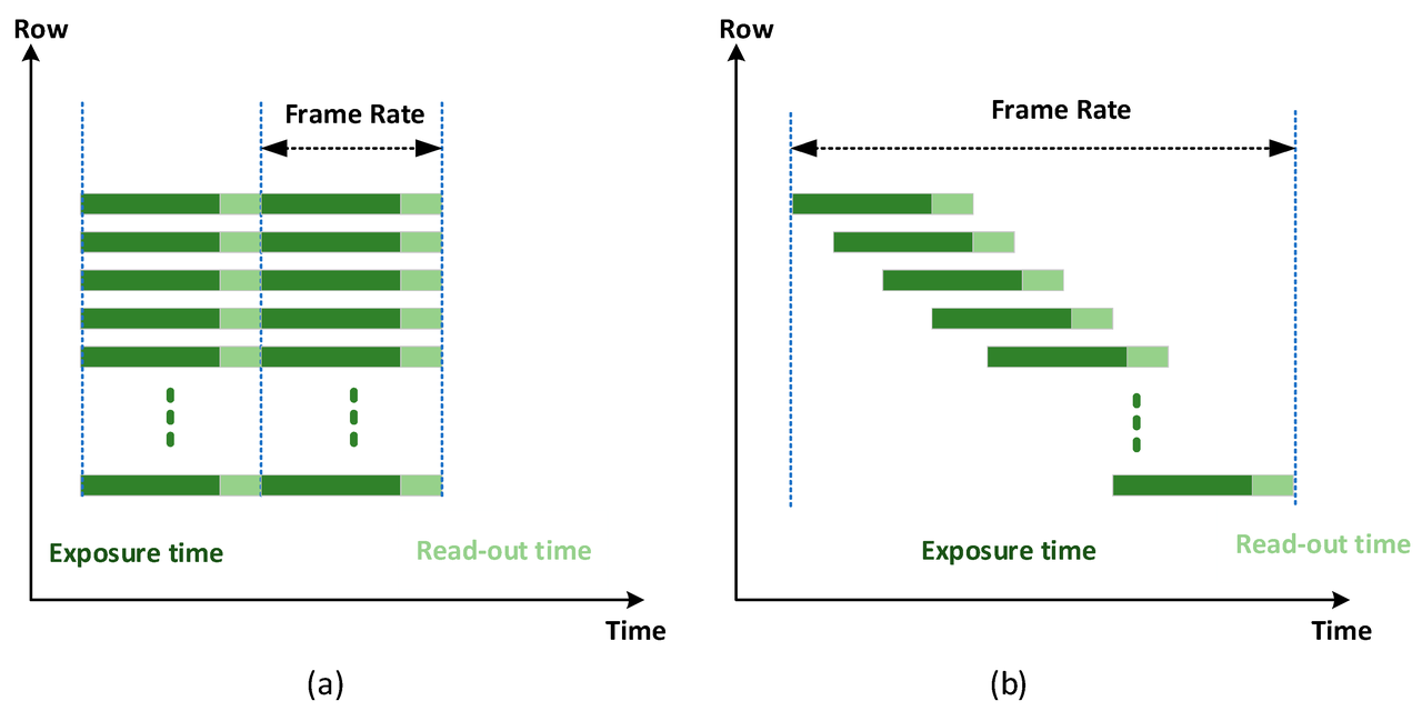
To efficiently capture and read the image, the time constraints for rolling shutter camera are:

1. The read-out time for each row is the same

2. The exposure time for each row is the same

3. The start of the read-out time of each row begins instantly after the end of the previous row’s read-out time

4. The exposure should start after the readout of the last frame

Warping Transformation for Undistortion

The warping transformation for undistorting is based on the same depth assumption [1].

The pixel of $^{c_n}\mathbf{q}_k$ captured by the rolling shutter camera at row $N$ can be transformed to the imaginary global shutter camera at the first row as follows:

$$^{c_0}\mathbf{q}_k = \frac{z_{c_n}}{z_{c_0}} \mathbf{K} \cdot {}^{c_0}\mathbf{T}_{c(n)} \cdot \mathbf{K}^{-1} \cdot {}^{c_n}\mathbf{q}_k$$

Usually, it is assumed that $z_{c_0} = z_{c_n}$, which simplifies above equation as follows:

$$^{c_0}\mathbf{q}_k = \mathbf{K} {}^{c_0}\mathbf{T}_{c(n)} \mathbf{K}^{-1} \cdot {}^{c_n}\mathbf{q}_k \tag{1}$$

This can be seen as a type of warp operation:

$$^{c_0}\mathbf{A}_{c(n)} = \mathbf{K} {}^{c_0}\mathbf{T}_{c(n)} \mathbf{K}^{-1}$$

and the equation (1) can be written as:

$$^{c_0}\mathbf{q}_k = {}^{c_0}\mathbf{A}_{c(n)} \cdot {}^{c_n}\mathbf{q}_k $$

where, the $^{c_0}\mathbf{A}_{c(n)}$ denotes the warp matrix projecting the pixel from the $c_{(n)}$ (exposure at time of line $n$) to the $c_0$ (exposure at time of line 0).

Rolling Shutter Projection

Problem Formulation

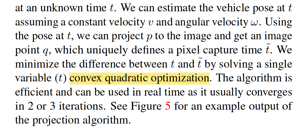
In [4], it says this estimation problem is a convex optimization problem. Let us break it down and figure out how to reach the conclusion.

Suppose a constant velocity, $v$, and angular velocity $w$ camera pose, then the pixel pose at time, $t$, relative to a pose, $\mathbf{T}_0$, is (using $T(3)\times SO(3)$ to represent the pose, $SE(3)$) [5]

$$\begin{aligned} \mathbf{T}_c(\delta t) &=\mathbf{T}_0\boxplus \mathbf{\tau}(\delta t)\\ &=\mathbf{T}_0 \begin{bmatrix} e^{[\delta t*w]_\times} & \delta t*v\\ 0 & 1 \end{bmatrix} \end{aligned}$$

We can project a point, $\mathbf{p}$, into the image plane and get its row numbers, $v$, as (here we use the pinhole camera model)

$$ \begin{bmatrix} x^c\\ y^c\\ z^c \end{bmatrix} = \mathbf{T}_c^{-1} \begin{bmatrix} x\\ y\\ z \end{bmatrix} ,\quad \begin{bmatrix} u\\ v\\ 1 \end{bmatrix} = \mathbf{K} \begin{bmatrix} x^c/z^c\\ y^c/z^c\\ 1 \end{bmatrix} $$

and the readout time at line $v$ is $t^\prime = t_0+v\Delta t$, where $t_0$ is the time in the first row and $\Delta t$ the readout time of each row. Minimizing the estimated time and the assumption time we get the problem formulation

$$ \underset{t}{\text{argmin}}\, \|t - t^\prime \left(K, \mathbf{T}(t), \mathbf{p}\right) \|^2 \tag{2} $$

where, $t$, can be interpreted as the relative time to the start of the first row.

Convexity Check

Let the LiDAR points, $\mathbf{p}$, undistorted to the time of the first row as, $\mathbf{x}$, we have, $\mathbf{x} = \mathbf{T}_0^{-1}\mathbf{p}$

Then points in the camera coordinate is,

$$\mathbf{x}^c = \begin{bmatrix} e^{[wt]_\times} & vt\\ 0 & 1 \end{bmatrix}^{-1} \mathbf{x}$$

where $t$ is the relative time to first row. Here

$$\begin{bmatrix} e^{[wt]_\times} & vt\\ 0 & 1 \end{bmatrix}^{-1}$$

can be approximated as

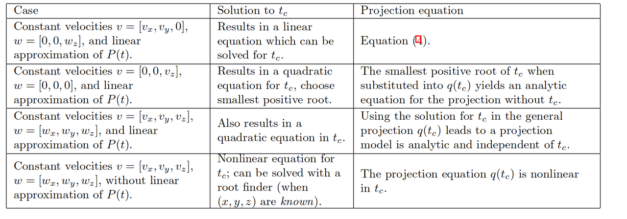
$$\begin{bmatrix} e^{[-wt]_\times} & -vt\\ 0 & 1 \end{bmatrix}$$

if we treat $SE(3)$ as composite of $\left< SO(3), \mathbb{R}^3 \right>$. Failed to prove it is convex. Can find the table below [3].

The Iterative Solution

We can also write the rolling shutter projection problem as a root finding problem [3]:

$$ t = t^\prime\left(K, \mathbf{T}(t), \mathbf{p}\right).\tag{3} $$

Then, we can resort to iterative algorithm by doing

$$ t_{k+1} = t^\prime\left(K, \mathbf{T}(t_k), \mathbf{p}\right). $$

The gap between problem (2) and (3) is that, the $t^\prime$ involves some integer operation, e.g., the projection on the pixel coordinate.

Then, the only problem is to prove the convergence of the iterative algorithm.

Convergence Proof for General Motion

The equation in (3) is a fixed-point problem. Its convergence does not depend on a particular camera-motion model, such as constant velocity. It only depends on how fast the projected image row changes during the rolling-shutter readout.

Let the valid readout interval of one image frame be

$$ I=[0,T_{\mathrm{rs}}], \qquad T_{\mathrm{rs}}=H\Delta t, $$

where $H$ is the image height and $\Delta t$ is the readout time per row. Let $\mathbf{T}(t)\in SE(3)$ be the camera pose at time $t\in I$. For a fixed world or LiDAR point $\mathbf{p}$, define its camera-frame coordinate as

$$ \mathbf{x}^c(t)= \begin{bmatrix} X(t)\\ Y(t)\\ Z(t) \end{bmatrix} =\mathbf{T}(t)^{-1}\mathbf{p}. $$

The continuous projected row is

$$ r(t)=c_y+f_y\frac{Y(t)}{Z(t)}. $$

For a standard top-to-bottom rolling-shutter sensor, after taking the first-row exposure time as the time origin, the row-readout map is

$$ \Phi(t)=\Delta t\,r(t). $$

More generally, one may write

$$ \Phi(t)=\tau(r(t)), $$

where $\tau$ maps an image row to its exposure time. For standard linear readout, $\tau(r)=\Delta t\,r$ and its Lipschitz constant is $L_\tau=\Delta t$. Reverse readout, cropped regions of interest, or nonuniform row timing can be handled by changing $\tau$; the proof below only needs $\tau$ to be Lipschitz.

The rolling-shutter projection time is a fixed point:

$$ t^\star=\Phi(t^\star).\tag{4} $$

Theorem. Consider one point $\mathbf{p}$ and one frame interval $I$. Assume that:

1. $\mathbf{T}(t)$ is continuously differentiable on $I$;

2. $Z(t)>0$ on $I$, so the perspective projection is well defined;

3. $\Phi(I)\subseteq I$, so the projected row corresponds to a valid exposure time inside the current frame;

4. the continuous row coordinate has bounded row velocity

   $$ M=\sup_{t\in I}|\dot r(t)|<\infty; $$

5. the row-time map $\tau$ is Lipschitz with constant $L_\tau$ and

   $$ q=L_\tau M<1.\tag{5} $$

Then $\Phi$ has a unique fixed point $t^\star\in I$. Moreover, the fixed-point iteration

$$ t^{(k+1)}=\Phi(t^{(k)}) $$

converges to $t^\star$ from any initial value $t^{(0)}\in I$. The convergence is geometric:

$$ |t^{(k)}-t^\star|\le q^k|t^{(0)}-t^\star|. $$

An equivalent a posteriori bound is

$$ |t^{(k)}-t^\star|\le \frac{q}{1-q}|t^{(k)}-t^{(k-1)}|. $$

Proof. Since $\mathbf{T}(t)$ is continuously differentiable and $Z(t)>0$ on the compact interval $I$, the row coordinate $r(t)$ is continuously differentiable on $I$. Therefore $r$ is Lipschitz with constant $M$. For any $t_1,t_2\in I$,

$$ \begin{aligned} |\Phi(t_1)-\Phi(t_2)| &=|\tau(r(t_1))-\tau(r(t_2))|\\ &\le L_\tau |r(t_1)-r(t_2)|\\ &\le L_\tau M |t_1-t_2|\\ &=q|t_1-t_2|. \end{aligned} $$

Because $q<1$, $\Phi$ is a contraction on $I$. Since $\Phi(I)\subseteq I$ and $I$ is complete, the Banach fixed-point theorem implies that $\Phi$ has a unique fixed point $t^\star\in I$ and that the iteration $t^{(k+1)}=\Phi(t^{(k)})$ converges to it for every initialization $t^{(0)}\in I$. Repeated application of the contraction inequality gives

$$ |t^{(k)}-t^\star| =|\Phi(t^{(k-1)})-\Phi(t^\star)| \le q|t^{(k-1)}-t^\star| \le q^k|t^{(0)}-t^\star|. $$

This proves the claim. $\square$

The derivative of the continuous projected row is

$$ \dot r(t) = f_y\frac{\dot Y(t)Z(t)-Y(t)\dot Z(t)}{Z(t)^2} =\frac{f_y}{Z(t)} \begin{bmatrix} 0 & 1 & -Y(t)/Z(t) \end{bmatrix} \dot{\mathbf{x}}^c(t).\tag{6} $$

Equation (6) is the key expression. It does not assume constant velocity, constant acceleration, or any particular trajectory parameterization. It only requires the camera-frame point trajectory $\mathbf{x}^c(t)$ to be differentiable.

If the instantaneous camera-frame twist is

$$ \boldsymbol{\xi}(t)=\left(\mathbf{v}(t),\boldsymbol{\omega}(t)\right), $$

where $\mathbf{v}(t)$ and $\boldsymbol{\omega}(t)$ are expressed in the camera frame, then for a static world point,

$$ \dot{\mathbf{x}}^c(t) =-\mathbf{v}(t)-\boldsymbol{\omega}(t)\times \mathbf{x}^c(t).\tag{7} $$

Substituting (7) into (6) gives

$$ \dot r(t) =\frac{f_y}{Z(t)} \begin{bmatrix} 0 & 1 & -Y(t)/Z(t) \end{bmatrix} \left(-\mathbf{v}(t)-\boldsymbol{\omega}(t)\times \mathbf{x}^c(t)\right). $$

Thus, for any time-varying translational and rotational motion pattern,

$$ M= \sup_{t\in I} \left| \frac{f_y}{Z(t)} \begin{bmatrix} 0 & 1 & -Y(t)/Z(t) \end{bmatrix} \left(-\mathbf{v}(t)-\boldsymbol{\omega}(t)\times \mathbf{x}^c(t)\right) \right|. $$

The iteration is guaranteed to converge whenever $L_\tau M<1$. For standard row-linear readout, this becomes

$$ \Delta t\,M<1. $$

Therefore, the sufficient convergence condition is not tied to the motion model itself. The condition is that the projected row moves by less than one image row during one row-readout interval. This covers constant velocity, constant acceleration, spline trajectories, IMU-integrated poses, and arbitrary smooth time-varying twists. If the point itself is moving, the same theorem still applies after replacing (7) by the actual relative derivative $\dot{\mathbf{x}}^c(t)=\frac{d}{dt}(\mathbf{T}(t)^{-1}\mathbf{p}(t))$.

A useful sufficient bound can be obtained from bounded relative motion. Let

$$ Z(t)\ge z_{\min}>0,\qquad \left|\frac{Y(t)}{Z(t)}\right|\le \eta_y, $$

and suppose

$$ \|\mathbf{v}(t)\|\le V,\qquad \|\boldsymbol{\omega}(t)\|\le \Omega,\qquad \frac{\|\mathbf{x}^c(t)\|}{Z(t)}\le \eta_x. $$

Then

$$ M \le f_y\sqrt{1+\eta_y^2} \left(\frac{V}{z_{\min}}+\Omega\eta_x\right). $$

Hence the following stronger but easier-to-check sufficient condition guarantees convergence:

$$ L_\tau f_y\sqrt{1+\eta_y^2} \left(\frac{V}{z_{\min}}+\Omega\eta_x\right)<1. $$

For standard linear readout, replace $L_\tau$ by $\Delta t$.

The proof above uses the continuous row coordinate $r(t)$. If the implementation applies $\lfloor r(t)\rfloor$, $\lceil r(t)\rceil$, or rounding inside the fixed-point iteration, the map becomes discontinuous, so Banach’s theorem no longer applies directly. A cleaner implementation is to iterate with the continuous row coordinate and quantize only after convergence.

If quantization must be applied inside the loop, let $Q$ be the quantizer and suppose

$$ |Q(r)-r|\le \epsilon_r. $$

For rounding, $\epsilon_r=1/2$ row; for floor or ceiling, $\epsilon_r<1$ row. The quantized update

$$ \tilde{\Phi}(t)=\tau(Q(r(t))) $$

is a bounded perturbation of the continuous contraction:

$$ |\tilde{\Phi}(t)-\Phi(t)|\le L_\tau\epsilon_r. $$

Therefore, relative to the continuous fixed point $t^\star$,

$$ |t^{(k+1)}-t^\star| \le q|t^{(k)}-t^\star|+L_\tau\epsilon_r. $$

Consequently, the quantized iteration is driven toward a neighborhood of the continuous solution whose asymptotic radius is bounded by

$$ \limsup_{k\to\infty}|t^{(k)}-t^\star| \le \frac{L_\tau\epsilon_r}{1-q}. $$

This bound explains why quantization usually causes at most a small row-level perturbation when $q$ is comfortably below one, but strict convergence of the quantized map is not guaranteed because discontinuities can introduce fixed-row jumps or short cycles.

The one-dimensional translation example is a special case. If there is no rotation, the depth is approximately constant, and the only relevant camera-frame velocity component is $v_y$, then

$$ M \approx f_y\frac{|v_y|}{z}, $$

and the standard-readout contraction condition becomes

$$ f_y\frac{|v_y|\Delta t}{z}<1. $$

For a 4K image with $f_y=1920$ and $\Delta t=1/(20\cdot2160)$, a velocity of $|v_y|=80$ gives

$$ f_y|v_y|\Delta t \approx 3.56. $$

Therefore, under this simplified worst-case motion, the fixed-point iteration is contractive for points with $z>3.56$. In practice, the vertical image-row velocity is often much smaller, so two or three iterations are usually enough. However, convergence is not unconditional: very close points, very fast vertical image motion, or strong rotations can violate $L_\tau M<1$.

Practical consideration: A LiDAR point is considered valid for the current rolling-shutter image only if the recovered camera exposure time lies inside the image capture interval. Let the camera frame start at $t_0$, and let the rolling-shutter readout interval be

$$ I_c=[t_0,t_0+H\Delta t]. $$

After solving the fixed-point problem, the point is accepted only if

$$ t^\star\in I_c,\qquad 0\le r(t^\star)0. $$

If $t^\star\notin I_c$, then the point has no physically valid observation in the current camera frame and should be rejected or projected into a neighboring camera frame. Clamping $t^\star$ to the interval boundary is not equivalent to rolling-shutter projection and may introduce artificial boundary correspondences.

Experiments

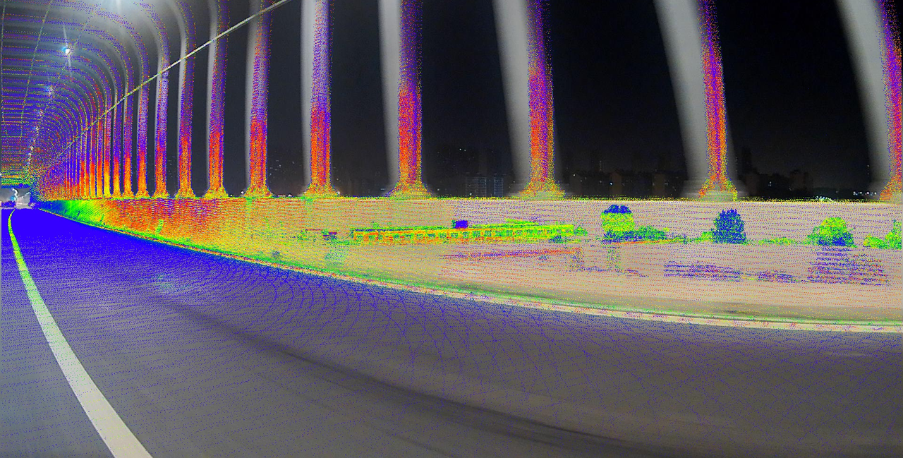
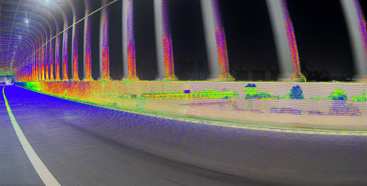
In this experiment, we project the LiDAR points onto the image plane with and without rolling shutter compensation [7]. From the figure, we can see that with rolling shutter compensation, the LiDAR points are more aligned with the image. However, we still need to compensate the exposure time to get more accurate results.

In real scenarios, we find two or three steps of iteration will lead convergent results.

References

[1] S. Hong, C. Zheng, H. Yin and S. Shen, “Rollvox: Real-Time and High-Quality LiDAR Colorization with Rolling Shutter Camera,” 2023 IEEE/RSJ International Conference on Intelligent Robots and Systems (IROS), Detroit, MI, USA, 2023, pp. 7195-7201, doi: 10.1109/IROS55552.2023.10342172.

[2] Li, You. “Spatial-Temporal Measurement Alignment of Rolling Shutter Camera and LiDAR.” IEEE Sensors Letters 6.12 (2022): 1-4.

[3] Meingast, Marci, Christopher Geyer, and Shankar Sastry. “Geometric models of rolling-shutter cameras.” arXiv preprint cs/0503076 (2005).

[4] Sun, Pei, et al. “Scalability in perception for autonomous driving: Waymo open dataset.” Proceedings of the IEEE/CVF conference on computer vision and pattern recognition. 2020.

[5] Sola, Joan, Jeremie Deray, and Dinesh Atchuthan. “A micro Lie theory for state estimation in robotics.” arXiv preprint arXiv:1812.01537 (2018).

[6] Li, Jingyi, and Weipeng Guan. 2018. “The Optical Barcode Detection and Recognition Method Based on Visible Light Communication Using Machine Learning” Applied Sciences 8, no. 12: 2425.

[7] Mao, Jiageng, Minzhe Niu, Chenhan Jiang, Hanxue Liang, Jingheng Chen, Xiaodan Liang, Yamin Li et al. “One million scenes for autonomous driving: Once dataset.” arXiv preprint arXiv:2106.11037 (2021).