In this post, we will discuss the Iterative Closest Point (ICP) problem: from point-to-point and point-to-plane ICP to generalized ICP.

Problem Formulation

Let two 3D point-sets $\mathcal{X} = \{\mathbf{x}_i\}, i = 1, \ldots, N$ and $\mathcal{Y} = \{\mathbf{y}_j\}, j = 1, \ldots, M$, where $\mathbf{x}_i, \mathbf{y}_j \in \mathbb{R}^3$ are point coordinates, be the data point-set and the model point-set respectively. The goal is to estimate a rigid motion with rotation $\mathbf{R} \in SO(3)$ and translation $\mathbf{t} \in \mathbb{R}^3$ that minimizes the following $L_2$-error $E$:

$$\underset{\mathbf{R}, \mathbf{t}}{\arg\min E(\mathbf{R}}, \mathbf{t}) = \sum_{i=1}^N e_i(\mathbf{R}, \mathbf{t})^2 = \sum_{i=1}^N \left\| \mathbf{R} \mathbf{x}_i + \mathbf{t} - \mathbf{y}_{j^*} \right\|^2 \tag{1}$$

where $e_i(\mathbf{R}, \mathbf{t})$ is the per-point residual error for $x_i$. Given $\mathbf{R}$ and $\mathbf{t}$, the point $y_{j^*} \in \mathcal{Y}$ is denoted as the optimal correspondence of $x_i$, which is the closest point to the transformed $x_i$ in $\mathcal{Y}$, i.e.,

$$j^* = \underset{j \in \{1, \ldots, M\}}{\arg \min} \left\| \mathbf{R} x_i + \mathbf{t} - \mathbf{y}_j \right\|\tag{2}$$

Note the short-hand notation used here: $j^*$ varies as a function of $(\mathbf{R}, \mathbf{t})$ and also depends on $x_i$.

Iterative closest point algorithm solves problem (1) by iteratively solving problem (1) and (2).

Iterative Solution

Solving the Problem with Fixed Pose

With fixed pose, problem (2) can be solved with a computational complexity of $\mathcal{O}(NM)$. However, we can build an octree to accelerate the closest point search. Further, if the data points are received sequentially, we can use an incremental kd-tree to update the tree [4].

Solving the Problem with Known Point Correspondence

With known point correspondence, problem (1) can be solved analytically.

$$\min_{\mathbf{R}\in SO(3), \mathbf{t}}\|\mathbf{R}\mathbf{x}_i+t-\mathbf{y}_i\|_2^2$$

For any $\mathbf{R}$, taking the derivative of the objective with respect to $\mathbf{t}$ and letting it equal to zero we have

$$\mathbf{t} = \frac{1}{N}\sum_i(\mathbf{y}_i - \mathbf{R}\mathbf{x}_i) = \bar{\mathbf{y}} - \mathbf{R}\bar{\mathbf{x}}$$

where we have $\bar{\mathbf{y}}\triangleq\frac{1}{N}\sum_i \mathbf{y}_i$ and $\bar{\mathbf{x}}\triangleq\frac{1}{N}\sum_i \mathbf{x}_i$. So, plug them into the objective function and let $\mathbf{x}_i\triangleq \mathbf{x}_i-\bar{\mathbf{x}}$ and $\mathbf{y}_i\triangleq \mathbf{y}_i - \bar{\mathbf{y}}$, we have

$$\min_{\mathbf{R}\in SO(3)} \|\mathbf{R}\mathbf{x}_i - \mathbf{y}_i\|_2^2$$

It is equivalent to

$$\max_{\mathbf{R}\in SO(3)}\,\mathbf{y}_i^\top\mathbf{R}\mathbf{x}_i$$

and further we have

$$\max_{\mathbf{R}\in SO(3)}\text{tr}(\mathbf{R}\sum_i \mathbf{x}_i\mathbf{y}_i^\top)$$

Let $\mathbf{M} = \sum_i \mathbf{x}_i\mathbf{y}_i^\top$. We are thus solving:

$$\max_{\mathbf{R}\in SO(3)}\text{tr}(\mathbf{R}\mathbf{M})$$

Let the SVD of $\mathbf{M} = \mathbf{U}\mathbf{\Sigma}\mathbf{V}^\top$. Then $\text{tr}(\mathbf{R}\mathbf{U}\mathbf{\Sigma}\mathbf{V}^\top) = \text{tr}(\mathbf{V}^\top\mathbf{R}\mathbf{U}\mathbf{\Sigma}) \triangleq \text{tr}(\mathbf{Q}\mathbf{\Sigma})$, where $\mathbf{Q}=\mathbf{V}^\top\mathbf{R}\mathbf{U}$ is an orthonormal matrix.

$$\text{tr}(\mathbf{Q}\mathbf{\Sigma}) = \sum_i q_{i,i}\sigma_{i}\leq \sum_i \sigma_{i}$$

The last equality holds when $q_{i,i}=1$ for all $i$ and $\sigma_{i,i}>0$, which means $\mathbf{Q}=\mathbf{I}$. Therefore, we have $\mathbf{R}=\mathbf{V}\mathbf{U}^\top$.

Since $SO(3)$ puts a determinant constraint on the orthonormal matrix with $\text{det}(R)=1$, we have two cases:

1. If $\text{det}(\mathbf{R})=1$, the optimal solution is $\mathbf{R}=\mathbf{V}\mathbf{U}^\top$.
2. If $\text{det}(\mathbf{R})=-1$, the algorithm fails.

In the case where $\text{det}(\mathbf{R})=-1$ and there exists at least one $\sigma_i$ that is zero, we can multiply $-1$ to its corresponding column of $\mathbf{U}$ or $\mathbf{V}$.

In the case where $\text{det}(\mathbf{R})=-1$ and all $\sigma_i$’s are positive, “This can happen only when the noises are very large. In that case, the least-squares solution is probably useless anyway. A better approach would be to use a RANSAC-like technique (using 3 points at a time) to combat against outliers” [1].

Other Variants of ICP

Let us first write the cost of problem (1) in a more general form:

$$ \underset{\mathbf{T}}{\text{argmin}} \sum_{i=1}^N \ell( \mathbf{T}\mathbf{x}_i, \mathbf{y}_{j^*}) $$

where $\mathbf{T} \in SE(3)$ and we have written the points in its homogeneous form.

Robust Point-to-point ICP

When there are outliers in the dataset or not every point has a corresponding correspondence, we can use a robust loss function $\ell$ to handle them. Typical choices are

$$ \ell(\mathbf{T}\mathbf{x}, \mathbf{y}) = w\|\mathbf{T}\mathbf{x}-\mathbf{y}\|_2^2 $$

where

$$ w = \begin{cases} 1, & \text{if } \|\mathbf{T}\mathbf{x}-\mathbf{y}\|_2 < d_{max} \\ 0, & \text{otherwise} \end{cases} $$

which means when the distance is larger than $d_{max}$, the point is considered an outlier and ignored.

Point to Plane ICP

The point-to-plane ICP is used as a more robust and accurate variant of the standard ICP. It minimizes the distance between the point and the plane [5]. The corresponding cost function is

$$ \ell(\mathbf{T}\mathbf{x}, \mathbf{y}) = \|w\cdot\mathbf{n}^\top(\mathbf{T}\mathbf{x}-\mathbf{y})\|_2^2 $$

where $\mathbf{n}$ is the normal vector of the plane where the point $\mathbf{y}$ is located.

Point-to-Line ICP

This variant is used when we know the target feature is a line. So, the cost function is the distance between the point and the line.

$$ \ell(\mathbf{T}\mathbf{x}, \mathbf{y}) = \|w\cdot(\mathbf{I} - \mathbf{n}\mathbf{n}^\top)(\mathbf{T}\mathbf{x}-\mathbf{y})\|_2^2 $$

where $\mathbf{n}$ is the unit direction vector of the line in which the point $\mathbf{y}$ is located.

Generalized ICP

Assume points $\{\mathbf{x}_i\}_{i=1}^N$ and $\{\mathbf{y}_i\}_{i=1}^N$ are already aligned, $\mathbf{x}_i\sim \mathcal{N}(\bar{\mathbf{x}}_i, \mathbf{C}^x_i)$ and $\mathbf{y}_i\sim \mathcal{N}(\bar{\mathbf{y}}_i, \mathbf{C}^y_i)$. Further, assume $\mathbf{y}_i = \mathbf{T}\mathbf{x}_i$. Thus, the residual, $\mathbf{d}^T_i = \mathbf{y}_i - \mathbf{T}\mathbf{x}_i$, is distributed as $\mathcal{N}(0, \mathbf{C}^y_i + \mathbf{T}\mathbf{C}^x_i\mathbf{T}^\top)$. Using the maximum log likelihood estimation, we have [6]

$$ \underset{\mathbf{T}}{\text{argmin}} \sum_{i=1}^N (\mathbf{d}_i^T)^\top\left(\mathbf{C}^y_i + \mathbf{T}\mathbf{C}^x_i\mathbf{T}^\top\right)^{-1}\mathbf{d}_i^T. \tag{3} $$

If we set $\mathbf{C}_i^x = \mathbf{0}$ and $\mathbf{C}_i^y =\mathbf{I}$, problem (3) is equivalent to the standard point-to-point ICP.

If we set $\mathbf{C}_i^x =\mathbf{0}$ and $\mathbf{C}_i^y = \mathbf{P}_i^{-1}$, where $\mathbf{P}_i$ is the projection onto the space spanned by the plane normal. Then, problem (3) is equivalent to the point-to-plane ICP. Also, we can construct the point-to-line ICP from the generalized ICP problem formulation.

Plane to Plane ICP

If the points are generated from a plane, we can assume that the points are generated from the distribution $\mathcal{N}(\bar{\mathbf{x}}, \mathbf{\Sigma})$, where

$$ \mathbf{\Sigma} = \mathbf{U} \begin{bmatrix} \mathbf{s_1} & \mathbf{0} & \mathbf{0} \\ \mathbf{0} & \mathbf{s_2} & \mathbf{0} \\ \mathbf{0} & \mathbf{0} & \mathbf{\epsilon} \end{bmatrix} \mathbf{U}^\top, $$

where $\epsilon$ should be a positive number near zero. By applying PCA on the point and along with its near by points, we can find such covariance matrix. Then, with the estimated covariance matrix, we can plug it into problem (3) to solve the generalized ICP problem, which is also called as the plane-to-plane ICP in [6]. In real practice, we should force $\mathbf{\Sigma}=\text{diag}(1, 1, \epsilon)$ to mitigate the effect of non uniformly distributed LiDAR points.

Normal Distributions Transform

The Normal Distributions Transform (NDT) method [7], published before Generalized ICP [6], offers an alternative approach to scan matching.

The NDT models the distribution of all reconstructed 2D-Points of one laser scan by a collection of local normal distributions. First, the 2D space around the robot is subdivided regularly into cells with constant size. Then for each cell, that contains at least three points, the following is done:

1. Collect all 2D-Points $\mathbf{x}_i$, $i = 1..n$, contained in this box.
2. Calculate the mean $\mathbf{q} = \frac{1}{n} \sum_i \mathbf{x}_i$.
3. Calculate the covariance matrix

$$ \Sigma = \frac{1}{n} \sum_i (\mathbf{x}_i - \mathbf{q})(\mathbf{x}_i - \mathbf{q})^t. $$

The probability of measuring a sample at 2D-point $\mathbf{x}$ contained in this cell is now modeled by the normal distribution $N(\mathbf{q}, \Sigma)$:

$$ p(\mathbf{x}) \sim \exp\left( -\frac{(\mathbf{x} - \mathbf{q})^t \Sigma^{-1} (\mathbf{x} - \mathbf{q})}{2} \right). $$

The outline of the proposed approach, given two scans (the first one and the second one), is as follows:

1. Build the NDT of the first scan.
2. Initialize the estimate for the parameters (by zero or by using odometry data).
3. For each sample of the second scan: Map the reconstructed 2D point into the coordinate frame of the first scan according to the parameters.
4. Determine the corresponding normal distributions for each mapped point.
5. The score for the parameters is determined by evaluating the distribution for each mapped point and summing the result.
6. Calculate a new parameter estimate by trying to optimize the score. This is done by performing one step of Newton’s Algorithm.
7. Go to step 3 until a convergence criterion is met.

The first four steps are straightforward: Building the NDT was described in the last section. As noted above, odometry data could be used to initialize the estimate. Mapping the second scan is done using $T$ and finding the corresponding normal distribution is a simple lookup in the grid of the NDT.

The rest is now described in detail using the following notation:

• $\mathbf{p} = (p_i)_{i=1..3} = (t_x, t_y, \phi)^t$: The vector of the parameters to estimate.
• $\mathbf{x}_i$: The reconstructed 2D point of laser scan sample $i$ of the second scan in the coordinate frame of the second scan.
• $\mathbf{x}_i'$: The point $\mathbf{x}_i$ mapped into the coordinate frame of the first scan according to the parameters $\mathbf{p}$, that is $\mathbf{x}_i' = T(\mathbf{x}_i, \mathbf{p})$.
• $\Sigma_i$, $\mathbf{q}_i$: The covariance matrix and the mean of the corresponding normal distribution to point $\mathbf{x}_i'$, looked up in the NDT of the first scan.

The mapping according to $\mathbf{p}$ could be considered optimal if the sum evaluating the normal distributions of all points $\mathbf{x}_i'$ with parameters $\Sigma_i$ and $\mathbf{q}_i$ is a maximum. We call this sum the score of $\mathbf{p}$. It is defined as:

$$ \text{score}(\mathbf{p}) = \sum_i \exp\left( -\frac{(\mathbf{x}_i' - \mathbf{q}_i)^t \Sigma_i^{-1} (\mathbf{x}_i' - \mathbf{q}_i)}{2} \right). $$

Finally, Newton’s method is applied iteratively to find the optimal parameters.

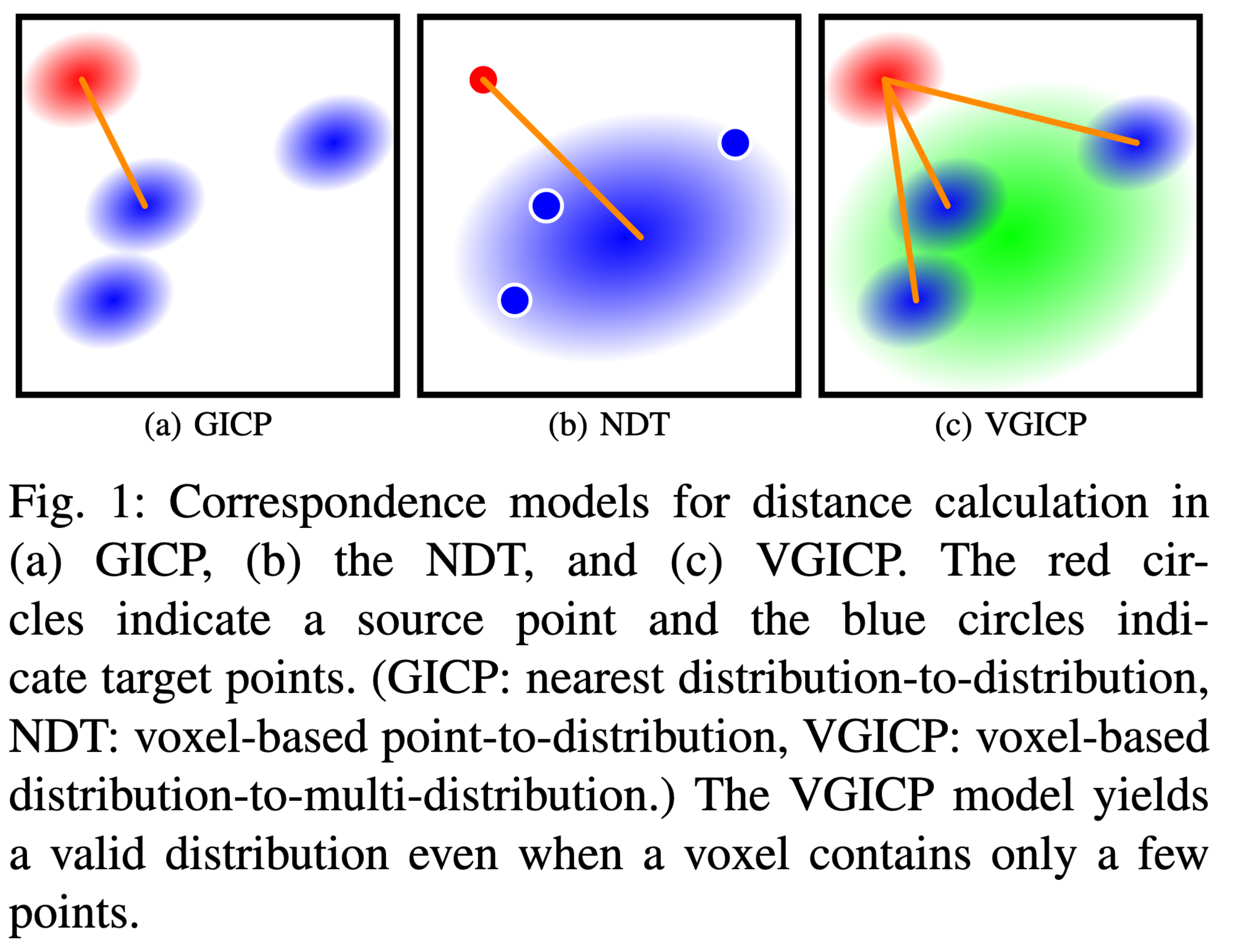
Voxelized GICP

Voxelized GICP [8] is built upon GICP [6]. It employs a point to multi-voxel mapping so that it eliminates the nearest neighbor search in the GICP. Then, it can efficiently compute the loss function by parallelizing the computation.

The following notation is similar to the one used in Eq. (3).

To derive the voxelized GICP algorithm, we first extend $\tilde{\mathbf{d}}_i$ so that it calculates the distances between $\mathbf{a}_i$ and its neighbor points $\{\mathbf{b}_j \mid \|\mathbf{a}_i - \mathbf{b}_j\| < r\}$ as follows:

$$ \tilde{\mathbf{d}}_i = \sum_j \left( \hat{\mathbf{b}}_j - \mathbf{T} \hat{\mathbf{a}}_i \right). $$

This equation can be interpreted as smoothing the target point distributions. Then, the distribution of $\tilde{\mathbf{d}}_i$ is given by

$$ \tilde{\mathbf{d}}_i \sim \left( \boldsymbol{\mu}^{\tilde{d}_i}, \mathbf{C}^{\tilde{d}_i} \right), $$$$ \mathbf{\mu}^{\tilde{d}_i} = \sum_j \left( \hat{\mathbf{b}}_j - \mathbf{T} \hat{\mathbf{a}}_i \right) = \mathbf{0}, $$$$ \mathbf{C}^{\tilde{d}_i} = \sum_j \left( \mathbf{C}^B_j + \mathbf{T} \mathbf{C}^A_i \mathbf{T}^T \right). $$

We estimate the transformation $\mathbf{T}$ that maximizes the log-likelihood of as follows:

$$ \mathbf{T} = \arg\min_\mathbf{T} \sum_i \left( \tilde{\mathbf{d}}_i^T \tilde{\mathbf{C}}_i^{-1} \tilde{\mathbf{d}}_i \right), $$

where

$$ \tilde{\mathbf{d}}_i = \sum_j \left( \mathbf{b}_j - \mathbf{T} \mathbf{a}_i \right), $$$$ \tilde{\mathbf{C}}_i = \sum_j \left( \mathbf{C}^B_j + \mathbf{T} \mathbf{C}^A_i \mathbf{T}^T \right). $$

To efficiently calculate the above equation, we modify it to:

$$ \mathbf{T} = \arg\min_\mathbf{T} \sum_i \left( N_i \tilde{\mathbf{d}}_i^T \tilde{\mathbf{C}}_i^{-1} \tilde{\mathbf{d}}_i \right), $$

where:

$$ \tilde{\mathbf{d}}_i = \frac{\sum_j \mathbf{b}_j}{N_i} - \mathbf{T} \mathbf{a}_i, $$$$ \tilde{\mathbf{C}}_i = \frac{\sum_j \mathbf{C}^B_j}{N_i} + \mathbf{T} \mathbf{C}^A_i \mathbf{T}^T. $$

where $N_i$ is the number of neighbor points. It suggests that we can efficiently compute the objective function by substituting the mean of the distributions of the points ($\mathbf{b}_j$ and $\mathbf{C}^B_j$) around $\mathbf{a}_i$ for $\mathbf{b}_i$ and $\mathbf{C}^B_i$ and weighting the function by $N_i$.

We can naturally adapt this equation to voxel-based calculation by storing $\mathbf{b}'_i = \frac{\sum \mathbf{b}_j}{N_i}$ and $\mathbf{C}'_i = \frac{\sum \mathbf{C}^B_j}{N_i}$ in each voxel.

Following the log-likelihood function, it uses Gauss-Newton method to optimize the objective function.

Performance Metrics

Information Matrix

The information matrix in the context of ICP is typically the Hessian matrix of the ICP cost function, which quantifies the curvature of the cost function at its minimum. This matrix, often a 6x6 matrix in 3D (corresponding to three translational and three rotational degrees of freedom), represents the precision or reliability of the estimated transformation parameters. In optimization, the Hessian is related to the Fisher information matrix, and its inverse provides the covariance matrix, indicating the uncertainty in the transformation estimate.

The information matrix is used to assess the reliability of the ICP alignment by providing an estimate of the uncertainty in the transformation parameters. A well-conditioned information matrix (with large diagonal elements) indicates high confidence in the transformation, suggesting that the point clouds are well-aligned with sufficient geometric constraints. Conversely, a poorly conditioned matrix (e.g., with small eigenvalues) suggests high uncertainty, possibly due to insufficient overlap, flat surfaces, or noisy data.

Fitness Score

The fitness score measures the overlap between the source and target point clouds, defined as the ratio of inlier correspondences (points within a maximum correspondence distance) to the total number of points in the target cloud. A higher fitness score suggests better alignment coverage.

Inlier RMSE

Inlier RMSE is the RMSE calculated only for inlier correspondences, providing a measure of alignment precision for the overlapping regions. It is expressed as:

$$ \text{Inlier RMSE} = \sqrt{\frac{1}{N_{\text{inliers}}} \sum_{i \in \text{inliers}} \|\mathbf{p}_i - \mathbf{q}_i\|^2} $$

where $N_{\text{inliers}}$ is the number of inliers. Lower values indicate higher precision.

Transformation Errors

When ground truth is available, transformation errors directly measure the accuracy of the estimated rotation and translation. These include:

1. Translation Error $e_t$: The Euclidean norm of the difference between estimated and true translation vectors:

$$ e_t = \sqrt{\Delta x^2 + \Delta y^2 + \Delta z^2} $$

2. Rotation Error $e_r$: The geodesic distance between estimated and true rotation matrices:

$$ e_r = \arccos\left(\frac{\text{trace}(\Delta \mathbf{R}) - 1}{2}\right) $$

Apppendix

Rotation Error Derivation

Below is a compact derivation that shows: why the shortest‐path (geodesic) rotation error between two rotation matrices is captured by

$$ e_r=\arccos\!\Bigl(\tfrac{\operatorname{tr}(\Delta \mathbf{R})-1}{2}\Bigr), \qquad \Delta \mathbf{R}:=\mathbf{R}_{\text{gt}}^{\top}\mathbf{R}_{\text{est}}\in\mathrm{SO}(3). $$

Distance on SO(3)

• $SO(3)$ is the Lie group of $3\times3$ rotation matrices.
• A natural, bi-invariant Riemannian metric gives a geodesic distance

$$ \begin{aligned} d(\mathbf{R}_1,\mathbf{R}_2) &=\|\log(\mathbf{R}_1^{\top}\mathbf{R}_2)\|_F/\sqrt{2}\\ &=\|\text{Log}(\mathbf{R}_1^{\top}\mathbf{R}_2)\|_2 \end{aligned} $$

where “$\log$” is the matrix logarithm sending a rotation to its axis–angle element of the Lie algebra $\mathfrak{so}(3)$ and “$\text{Log}$” is the matrix logarithm sending a rotation to its vector space.

For $\Delta \mathbf{R}\in\mathrm{SO}(3)$ there exists an axis $\mathbf{u}\in\mathbb{S}^2$ and angle $\theta\in[-\pi,\pi]$ such that

$$ \Delta \mathbf{R}=\exp\bigl(\,[\mathbf{u}]_\times\,\theta\bigr) \quad\Rightarrow\quad \log(\Delta R)=[\mathbf{u}]_\times\theta, $$

so the Frobenius norm of the log is $\|[\mathbf{u}]_\times\theta\|_F=\sqrt{2}\,|\theta|$. Hence $d(\mathbf{R}_1,\mathbf{R}_2)=|\theta|$. The distance is exactly the rotation angle $\theta$.

Relating the Angle $\theta$ to the Trace

Start with Rodrigues’ formula for any $\theta$ and unit axis $\mathbf{u}$:

$$ \exp\bigl([\mathbf{u}]_\times\theta\bigr) =I+\sin\theta\,[\mathbf{u}]_\times +(1-\cos\theta)\,[\mathbf{u}]_\times^{2}. $$

Taking the trace and using $\operatorname{tr}([\mathbf{u}]_\times)=0$ and $\operatorname{tr}([\mathbf{u}]_\times^{2})=-2$:

$$ \operatorname{tr}(\Delta \mathbf{R})=\operatorname{tr}(\mathbf{I})+0+(-2)(1-\cos\theta) =1+2\cos\theta. $$

Solve for $\theta$:

$$ \cos\theta=\tfrac{\operatorname{tr}(\Delta \mathbf{R})-1}{2} \quad\Longrightarrow\quad \theta=\arccos\!\Bigl(\tfrac{\operatorname{tr}(\Delta \mathbf{R})-1}{2}\Bigr). $$

Putting it together

• Compute the relative rotation $\Delta \mathbf{R}=\mathbf{R}_{\text{gt}}^{\top}\mathbf{R}_{\text{est}}$ . (Because the metric is right-invariant, left–multiplying both rotations by the same matrix has no effect.)
• Extract the rotation angle with the trace formula above.
• That angle is the geodesic distance on $SO(3)$, so we call it the rotation error $e_r$.

Useful Properties

• Invariance: $e_r\bigl(\mathbf{Q}\mathbf{R}_{\text{gt}},\,\mathbf{Q}\mathbf{R}_{\text{est}}\bigr)=e_r(\mathbf{R}_{\text{gt}},\mathbf{R}_{\text{est}})$ for any $\mathbf{Q}\in SO(3)$.
• Range: trace $(\Delta R)\in[-1,3] \Rightarrow e_r\in[0,\pi]$.
• Small-angle limit: when $\theta\!\ll\!1$, $e_r\approx\|\mathbf{r}\|_2$ where $\mathbf{r}$ is the 3-vector in the Lie-algebra log.

Thus the trace-based formula is simply a closed-form way of reading off the minimal rotation angle between two orientations, which is exactly the geodesic distance on the manifold of rotations.

Information Matrix Derivation

Definition of the Information Matrix

The information matrix in ICP is typically the Hessian matrix of the cost function, which quantifies the curvature of the cost function at its minimum. This $6 \times 6$ matrix corresponds to the six degrees of freedom in 3D rigid transformations (three for rotation, three for translation). In estimation theory, it is related to the Fisher information matrix, and its inverse provides the covariance matrix, indicating the uncertainty in the transformation estimate. A well-conditioned information matrix (with large eigenvalues) suggests high confidence in the alignment, while a poorly conditioned matrix indicates potential ambiguities, such as in featureless environments. [10]

Theoretical Foundation

The information matrix is derived from the Hessian of the ICP cost function. For least squares problems, the cost function is of the form

$$ f = \frac{1}{2} \sum_i \|\mathbf{r}_i(\boldsymbol{\theta})\|^2 $$

where $\mathbf{r}_i$ is the residual for each correspondence and $\boldsymbol{\theta}$ is the optimization variable. Take second derivative of the cost function with respect to the optimization variable, we have:

$$ \begin{aligned} \nabla^2_{\boldsymbol{\theta}} f &= \nabla_{\boldsymbol{\theta}}\left( \sum_i \nabla_{\boldsymbol{\theta}} \mathbf{r}_i \cdot \mathbf{r}_i \right) \\ &= \sum_i \nabla^2_{\boldsymbol{\theta}} \mathbf{r}_i \cdot \mathbf{r}_i + \sum_i \nabla_{\boldsymbol{\theta}} \mathbf{r}_i \nabla_{\boldsymbol{\theta}} \mathbf{r}_i^T \end{aligned} $$

when $\mathbf{r}_i$ is approximately zero, the Hessian matrix is:

$$ \mathbf{H} = \nabla^2_{\boldsymbol{\theta}} f \approx \sum_i \nabla_{\boldsymbol{\theta}} \mathbf{r}_i \nabla_{\boldsymbol{\theta}} \mathbf{r}_i^T =\mathbf{J}^\top \mathbf{J} $$

where $\mathbf{J}$ is the Jacobian of the residuals with respect to the transformation parameters.

Note: the Jacobian is defined as $\mathbf{J} = \nabla_{\boldsymbol{\theta}} \mathbf{r}_i^\top$. The shape differs from traditional matrix calculus textbook.

In ICP, the transformation is parameterized by a 6-vector $\xi = (\boldsymbol{\omega}, \mathbf{t})$, where $\boldsymbol{\omega}$ represents the rotation (often as a rotation vector for small angles) and $\mathbf{t}$ is the translation.

Point-to-Point ICP Cost Function

For point-to-point ICP, the cost function is:

$$ f = \sum_i \| \mathbf{R} \mathbf{p}_i + \mathbf{t} - \mathbf{q}_i \|^2 $$

where $\mathbf{p}_i$ are source points, $\mathbf{q}_i$ are target points, and $\mathbf{R}$ and $\mathbf{t}$ are the rotation matrix and translation vector. Let us represent the rotation as, $\mathbf{R} = \exp([\boldsymbol{\omega}]_\times) \mathbf{R}_0$ with an already obtained rotation matrix $\mathbf{R}_0$ and a small perturbation, $\boldsymbol{\omega} \in \mathbb{R}^3$, around it, and $[\boldsymbol{\omega}]_\times$ is the skew-symmetric matrix. (Here we can also use right perturbation, $\mathbf{R} = \mathbf{R}_0 \exp([\boldsymbol{\omega}]_\times)$. But for iterative optimization method, right perturbation is preferred. For right perturbation, you can compute $\mathbf{R}_0\mathbf{p}_i$ iteratively. When an updating is made, we can re-use the previous $\mathbf{R}_0\mathbf{p}_i$ to compute the new $\mathbf{R}_0\mathbf{p}_i$. However, for IMU, we use right perturbation $\dot{\mathbf{R}} = \mathbf{R}[\boldsymbol{\omega}]_\times$.) By expanding the matrix exponential and omit the higher order terms, we have, $\mathbf{R} \approx (\mathbf{I} + [\boldsymbol{\omega}]_\times) \mathbf{R}_0$. The residual for each correspondence is:

$$ r_i = \mathbf{R} \mathbf{p}_i + \mathbf{t} - \mathbf{q}_i \approx \mathbf{R}_0\mathbf{p}_i - \mathbf{q}_i + \mathbf{t} + [\boldsymbol{\omega}]_\times\mathbf{R}_0\mathbf{p}_i $$

Since $[\boldsymbol{\omega}]_\times \mathbf{R}_0 \mathbf{p}_i = \boldsymbol{\omega} \times (\mathbf{R}_0 \mathbf{p}_i) = - \mathbf{R}_0 \mathbf{p}_i \times \boldsymbol{\omega} = - [\mathbf{R}_0 \mathbf{p}_i]_\times \boldsymbol{\omega}$, we have:

$$ r_i \approx (\mathbf{R}_0\mathbf{p}_i - \mathbf{q}_i) + \mathbf{t} - [\mathbf{R}_0 \mathbf{p}_i]_\times \boldsymbol{\omega}. $$

So, the Jacobian $\mathbf{J}_i = [\frac{\partial \mathbf{r}_i}{\partial \boldsymbol{\omega}}, \frac{\partial \mathbf{r}_i}{\partial \mathbf{t}}]$ is:

$$ \mathbf{J}_i = \begin{bmatrix} -[\mathbf{R}_0 \mathbf{p}_i]_\times & \mathbf{I}_3 \end{bmatrix} $$

Hence, the Hessian is:

$$ \begin{aligned} \mathbf{H} &= \sum_i \mathbf{J}_i^T \mathbf{J}_i \\ &= \begin{bmatrix} \sum_i [\mathbf{R}_0 \mathbf{p}_i]_\times^T [\mathbf{R}_0 \mathbf{p}_i]_\times & \sum_i [\mathbf{R}_0 \mathbf{p}_i]_\times^T \\ \sum_i [\mathbf{R}_0 \mathbf{p}_i]_\times & \sum_i \mathbf{I}_3 \end{bmatrix}. \end{aligned} $$

The Hessian with the translation is always constant and the correlation between the rotation and translation is $\sum_i [\mathbf{R}_0 \mathbf{p}_i]_\times$. The Hessian for the rotation is $\sum_i [\mathbf{R}_0 \mathbf{p}_i]_\times^T [\mathbf{R}_0 \mathbf{p}_i]_\times$. Here, we are particularly interested in the rotation part.

Since $[\boldsymbol{\omega}]_\times^\top = -[\boldsymbol{\omega}]_\times$, and $[\boldsymbol{\omega}]_\times^2 = \boldsymbol{\omega} \boldsymbol{\omega}^\top - \|\boldsymbol{\omega}\|^2 \mathbf{I}$. Therefore, the Hessian for the rotation is

$$ \mathbf{H}_{\boldsymbol{\omega}} = \sum_i \left( \|\mathbf{p}_i\|^2 \mathbf{I} - \mathbf{R}_0 \mathbf{p}_i (\mathbf{R}_0 \mathbf{p}_i)^\top \right). $$

Let $\mathbf{x}_i = \mathbf{R}_0 \mathbf{p}_i$, then the Hessian for the rotation is

$$ \mathbf{H}_{\boldsymbol{\omega}} = \sum_i \left( \|\mathbf{x}_i\|^2 \mathbf{I} - \mathbf{x}_i \mathbf{x}_i^\top \right). $$

First, we should note that the Hessian is semi-positive definite by definition. A “good” Hessian should have

1. The smallest eigenvalue is large
2. The condition number is close to 1

Note also that $\sum_i \|\mathbf{x}_i\|^2 \mathbf{I} - \sum_i \mathbf{x}_i \mathbf{x}_i^\top$ is the null space of the space spanned by $\{\mathbf{x}_i\}$. To satisfy the first condition, we need at least three points that not collinear or in the same plane. The second condition inspires us to distribute the points as evenly as possible.

Point-to-Plane ICP Cost Function

For point-to-plane ICP, the cost function is:

$$ f = \frac{1}{2} \sum_i \left( \mathbf{n}_i^\top (\mathbf{R} \mathbf{p}_i + \mathbf{t} - \mathbf{q}_i) \right)^2 $$

where $\mathbf{n}_i$ is the surface normal at $\mathbf{q}_i$. The residual is:

$$ \mathbf{r}_i = \mathbf{n}_i^T (\mathbf{R} \mathbf{p}_i + \mathbf{t} - \mathbf{q}_i) $$

For small rotations $\exp([\boldsymbol{\omega}]_\times)$ around $\mathbf{R}_0$, $\mathbf{R} \mathbf{p}_i \approx \mathbf{R}_0 \mathbf{p}_i + [\boldsymbol{\omega}]_\times \mathbf{R}_0 \mathbf{p}_i$, so:

$$ \mathbf{r}_i \approx \mathbf{n}_i^T (\mathbf{R}_0 \mathbf{p}_i + [\boldsymbol{\omega}]_\times \mathbf{R}_0 \mathbf{p}_i + \mathbf{t} - \mathbf{q}_i) $$

The Jacobian is:

$$ \mathbf{J}_i = \begin{bmatrix} -\mathbf{n}_i^\top[\mathbf{R}_0\mathbf{p}_i]_\times & \mathbf{n}_i^T \end{bmatrix} $$

Let $\mathbf{x}_i = \mathbf{R}_0 \mathbf{p}_i$, then the Hessian is:

$$ \begin{aligned} \mathbf{H} &= \sum_i \mathbf{J}_i^T \mathbf{J}_i \\ &= \begin{bmatrix} \sum_i [\mathbf{x}_i]_\times^T \mathbf{n}_i \mathbf{n}_i^T [\mathbf{x}_i]_\times & -\sum_i [\mathbf{x}_i]_\times^T \mathbf{n}_i \mathbf{n}_i^\top\\ -\sum_i \mathbf{n}_i\mathbf{n}_i^\top[\mathbf{x}_i]_\times & \sum_i \mathbf{n}_i \mathbf{n}_i^\top \end{bmatrix} \end{aligned} $$

For the translation part, $\mathbf{H}_{\mathbf{t}} = \sum_i \mathbf{n}_i \mathbf{n}_i^\top$, remember the length of the normal vector is 1, i.e., $\|\mathbf{n}_i\| = 1$, and $\sum_i \mathbf{n}_i \mathbf{n}_i^\top$ is the space spanned by $\{\mathbf{n}_i\}$. Thus, a good Hessian indicates that the normal vectors should spatial evenly distributed.

For the rotation part, $\mathbf{H}_{\boldsymbol{\omega}} = \sum_i [\mathbf{x}_i]_\times^T \mathbf{n}_i \mathbf{n}_i^T [\mathbf{x}_i]_\times$. Let $\boldsymbol{\nu}_i = [\mathbf{x}_i]_\times\mathbf{n}_i = \mathbf{x}_i \times \mathbf{n}_i$, we have

$$ \mathbf{H}_{\boldsymbol{\omega}} = \sum_i \boldsymbol{\nu}_i\boldsymbol{\nu}_i^\top. $$

This Hessian is the space spanned by $\{\boldsymbol{\nu}_i\}$. Since $\boldsymbol{\nu}_i$ is the cross product of $\mathbf{x}_i$ and $\mathbf{n}_i$, it is perpendicular to both $\mathbf{x}_i$ and $\mathbf{n}_i$. Thus, a good Hessian requires the normal of the plane spanned by pairs of $\mathbf{x}_i$ and $\mathbf{n}_i$ are evenly distributed. It is also intuitive that the points along the normal direction contribute no information to the rotation.

Point-to-Line ICP Cost Function

For point-to-line ICP, the cost function is:

$$ f = \frac{1}{2} \sum_i \left\| (\mathbf{I} - \mathbf{n}_i\mathbf{n}_i^\top)(\mathbf{R} \mathbf{p}_i + \mathbf{t} - \mathbf{q}_i) \right\|^2 $$

where $\mathbf{n}_i$ is the direction unit vector of the line. The residual is:

$$ \mathbf{r}_i = (\mathbf{I} - \mathbf{n}_i\mathbf{n}_i^\top)(\mathbf{R} \mathbf{p}_i + \mathbf{t} - \mathbf{q}_i) $$

Follow similar steps as before, the Jacobian is:

$$ \mathbf{J}_i = \begin{bmatrix} -(\mathbf{I} - \mathbf{n}_i\mathbf{n}_i^\top)[\mathbf{R}_0\mathbf{p}_i]_\times & \mathbf{I} - \mathbf{n}_i\mathbf{n}_i^\top \end{bmatrix} $$

Let $\mathbf{x}_i = \mathbf{R}_0 \mathbf{p}_i$, then the Hessian is:

$$ \begin{aligned} \mathbf{H} &= \sum_i \mathbf{J}_i^T \mathbf{J}_i \\ &= \begin{bmatrix} \sum_i [\mathbf{x}_i]_\times^T (\mathbf{I} - \mathbf{n}_i\mathbf{n}_i^\top) [\mathbf{x}_i]_\times & \sum_i [\mathbf{x}_i]_\times^T (\mathbf{I} - \mathbf{n}_i\mathbf{n}_i^\top) \\ \sum_i (\mathbf{I} - \mathbf{n}_i\mathbf{n}_i^\top) [\mathbf{x}_i]_\times & \sum_i (\mathbf{I} - \mathbf{n}_i\mathbf{n}_i^\top) \end{bmatrix} \end{aligned} $$

This problem is like the dual of the point-to-plane ICP, where $\mathbf{I}-\mathbf{n}_i\mathbf{n}_i^\top$ is the projection matrix onto the plane orthogonal to $\mathbf{n}_i$. So, for the translation part, a good Hessian requires of the normal vectors are evenly distributed in the unit sphere.

For the rotation part, the Hessian is:

$$ \begin{aligned} \mathbf{H}_{\boldsymbol{\omega}} &= \sum_i [\mathbf{x}_i]_\times^T (\mathbf{I} - \mathbf{n}_i\mathbf{n}_i^\top) [\mathbf{x}_i]_\times \\ &= \sum_i \left( [\mathbf{x}_i]_\times^T [\mathbf{x}_i]_\times - [\mathbf{x}_i]_\times^T \mathbf{n}_i \mathbf{n}_i^\top[\mathbf{x}_i]_\times \right)\\ &=\sum_i \left( \|\mathbf{x}_i\|^2 \mathbf{I} - \mathbf{x}_i \mathbf{x}_i^\top - \mathbf{u}_i\mathbf{u}_i^\top \right)\\ &=\sum_i \|\mathbf{x}_i\|^2 \left( \mathbf{I} - \mathbf{v}_i \mathbf{v}_i^\top - (\mathbf{v_i\times \mathbf{n}_i})(\mathbf{v_i\times \mathbf{n}_i})^\top \right) \end{aligned} $$

where $\mathbf{u}_i = \mathbf{x}_i \times \mathbf{n}_i$ is the cross product of $\mathbf{x}_i$ and $\mathbf{n}_i$ and $\mathbf{v}_i = \frac{\mathbf{x}_i}{\|\mathbf{x}_i\|}$ is the unit vector of $\mathbf{x}_i$. Then, a good Hessian requires that

1. The length of $\mathbf{x}_i$ is large
2. The length of $\mathbf{x}_i$ is similar
3. $\mathbf{x}_i$ is spatially evenly distributed
4. The length of $\mathbf{u}_i$ is similar
5. The normal vectors of the planes spanned by $\mathbf{x}_i$ and $\mathbf{n}_i$ are evenly distributed, then $\mathbf{n}_i$ is spatially evenly distributed

References

[1] K. S. Arun, T. S. Huang, and S. D. Blostein, “Least-Squares Fitting of Two 3-D Point Sets,” IEEE Trans. Pattern Anal. Mach. Intell., vol. PAMI-9, no. 5, pp. 698–700, Sep. 1987, doi: 10.1109/TPAMI.1987.4767965.

[2] Y. Zheng, Y. Kuang, S. Sugimoto, K. Astrom, and M. Okutomi, “Revisiting the PnP Problem: A Fast, General and Optimal Solution,” in 2013 IEEE International Conference on Computer Vision, Sydney, Australia: IEEE, Dec. 2013, pp. 2344–2351. doi: 10.1109/ICCV.2013.291.

[3] G. Terzakis and M. Lourakis, “A Consistently Fast and Globally Optimal Solution to the Perspective-n-Point Problem,” in Computer Vision – ECCV 2020, vol. 12346, A. Vedaldi, H. Bischof, T. Brox, and J.-M. Frahm, Eds., in Lecture Notes in Computer Science, vol. 12346. , Cham: Springer International Publishing, 2020, pp. 478–494. doi: 10.1007/978-3-030-58452-8_28.

[4] Y. Cai, W. Xu, and F. Zhang, “ikd-Tree: An Incremental K-D Tree for Robotic Applications,” arXiv preprint arXiv:2102.10808, 2021.

[5] Y. Chen and G. Medioni, “Object modelling by registration of multiple range images,” Image and Vision Computing, vol. 10, no. 3, pp. 145–155, Apr. 1992, doi: 10.1016/0262-8856(92)90066-C

[6] Segal, Aleksandr, Dirk Haehnel, and Sebastian Thrun. “Generalized-icp.” Robotics: science and systems. Vol. 2. No. 4. 2009.

[7] P. Biber and W. Strasser, “The normal distributions transform: a new approach to laser scan matching,” in Proceedings 2003 IEEE/RSJ International Conference on Intelligent Robots and Systems (IROS 2003) (Cat. No.03CH37453), Las Vegas, Nevada, USA: IEEE, 2003, pp. 2743–2748. doi: 10.1109/IROS.2003.1249285.

[8] K. Koide, M. Yokozuka, S. Oishi, and A. Banno, “Voxelized GICP for Fast and Accurate 3D Point Cloud Registration,” in 2021 IEEE International Conference on Robotics and Automation (ICRA), Xi’an, China: IEEE, May 2021, pp. 11054–11059. doi: 10.1109/ICRA48506.2021.9560835.

[9] J. Zhang, Y. Yao, and B. Deng, “Fast and robust iterative closest point,” IEEE Transactions on Pattern Analysis and Machine Intelligence, vol. 44, no. 7, pp. 3450–3466, Jul. 2022, doi: 10.1109/TPAMI.2021.3054619.

[10] S. Choi, Q.-Y. Zhou, and V. Koltun, “Robust reconstruction of indoor scenes,” in Proceedings of the IEEE Conference on Computer Vision and Pattern Recognition (CVPR), Boston, MA, USA, 2015, pp. 5556–5565, doi: 10.1109/CVPR.2015.7299195.

[11] M. Barczyk and S. Bonnabel, “Observability, covariance and uncertainty of ICP-based scan-matching,” 2014 IEEE/RSJ International Conference on Intelligent Robots and Systems (IROS), Chicago, IL, USA, 2014, pp. 1760–1765, doi: 10.1109/IROS.2014.6942762.

[12] S. Bonnabel, M. Barczyk and F. Goulette, “On the covariance of ICP-based scan-matching techniques,” 2016 American Control Conference (ACC), Boston, MA, USA, 2016, pp. 5498-5503, doi: 10.1109/ACC.2016.7526532.